topic badge

9.03 Normal distributions

Introduction

In Algebra 1 lesson  7.03 Measures of spread  , we learned how the mean and standard deviation of a data set affect its distribution. In Algebra 1 lesson,  7.04 Interpreting data distributions  , we learned how to describe the shape of a data distribution. We will use concepts from those lessons to identity symmetric distributions. In this lesson, we will learn special properties related to symmetric distributions.

Normal distribution

A data set that is symmetric and bell-shaped about the mean is said to have an approximately normal distribution.

A histogram with Percentage on the y-axis, with numbers 0 through 30, and Weight on the x-axis, with bars labeled at their endpoint 75 to 110 in steps of 5. The heights of the bars follow a bell shape with its peak at the 90 through 95 bar. A curve is also plotted with a mound on the middle and tails trailing off to the left and right.

This shows how a data set that has an approximately normal distribution may appear in a histogram. The dark line shows the nice, symmetrical curve that can be drawn over the histogram that the data roughly follows.

In the distribution above, the peak of the data represents the mean, the median, and the mode. All these measures of central tendency are equal for this symmetrical distribution.

If a data set is not symmetrical about the mean, we cannot use normal distribution to interpret it. Recall from Algebra 1 that data sets that are not symmetric are skewed.

A histogram with Relative Frequency on the y-axis and Score on the x-axis. The are 8 bars in the histogram. The heights of the bars follow a bell shape with its peak at the third leftmost bar and a steady decrease in the bar heights on the right. A curve is plotted with a mound on the left and a tail trailing off to the right.
Skewed right
A histogram with Relative Frequency on the y-axis and Score on the x-axis. The are 8 bars in the histogram. The heights of the bars follow a bell shape with its peak at the third rightmost bar and a steady decrease in the bar heights on the left. A curve is plotted with a mound on the right and a tail trailing off to the left.
Skewed left

The shape of the normal distribution will depend on the population parameters: the mean, denoted by \mu, and the standard deviation, denoted by \sigma. The standard deviation describes the spread of the data.

-1
1
x
1
y
A small standard deviation provides a tight cluster around the mean
-1
1
x
1
y
A larger standard deviation shows data that is more spread out

Exploration

  1. Match each of the histograms pictured below to the correct mean and standard deviation.

  2. Justify your choices.

  • \mu=16, \sigma=3
  • \mu=15,\sigma=2
  • \mu=19,\sigma=4
  • \mu=18,\sigma=2
A histogram with numbers 7 to 31, in steps of 4, on the x axis. The heights of the bars follow a bell shape with its peak at the 19 mark. Speak to your teacher for more details.
Histogram 1
A histogram with numbers 8 to 22, in steps of 2, on the x axis. The heights of the bars follow a bell shape with its peak between the 14 to 16 mark. Speak to your teacher for more details.
Histogram 2
A histogram with numbers 12 to 24, in steps of 2, on the x axis. The heights of the bars follow a bell shape with its peak around the 18 mark. Speak to your teacher for more details.
Histogram 3
A histogram with numbers 5 to 40, in steps of 5, on the x axis. There are bars from around the 5 mark to around the 25 mark. The heights of the bars follow a bell shape with its peak just after the 15 mark. Speak to your teacher for more details.
Histogram 4

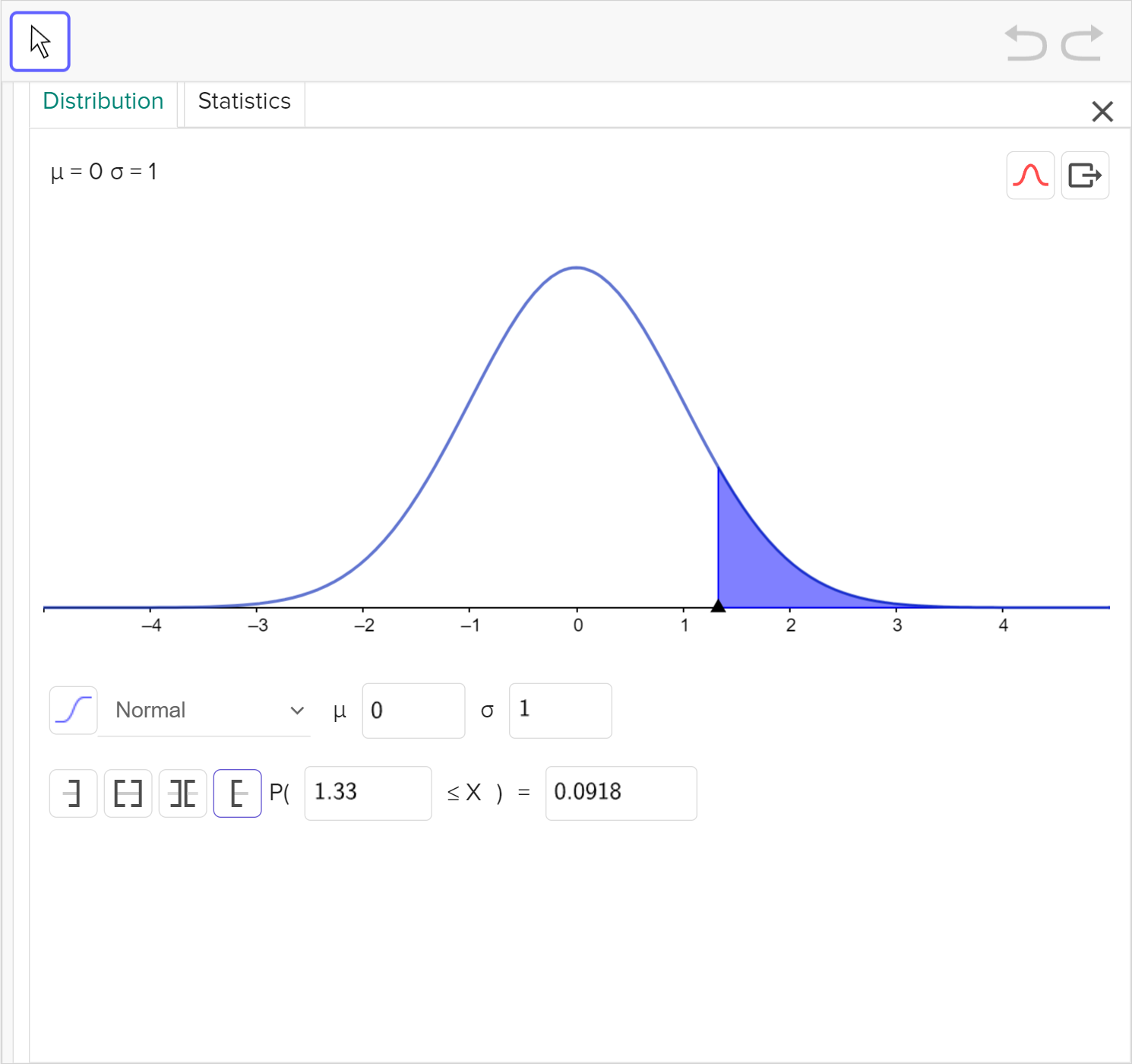
In a density curve, the area beneath the curve represents probability with the area under the entire curve equal to 100\%, or 1. When data is approximately normally distributed, the probability between 1, 2, and 3 standard deviations can be accurately summarized using the empirical rule.

A normal distribution curve. Below the curve is a horizontal axis with the following evenly spaced marks from left to right: mu minus 3 sigma, mu minus 2 sigma, mu minus sigma, mu, mu plus sigma, mu plus 2 sigma, and mu plus 3 sigma. The peak of the curve is at mu. Vertical lines are drawn from the curve to each mark in the horizontal axis. The area under the curve between the mu minus 3 sigma and mu minus 2 sigma is labeled 2.35 percent, between mu minus 2 sigma and mu minus sigma labeled 13.5 percent, between mu minus sigma and mu labeled 34 percent, between mu and mu plus sigma labeled 34 percent, between mu plus sigma and mu plus 2 sigma labeled 13.5 percent, and between mu plus 2 sigma and mu plus 3 sigma labeled 2.35 percent. Below the horizontal axis, a set of three brackets labeled Empirical rule are shown: a bracket connecting mu minus sigma and mu plus sigma is labeled 68 percent, a bracket connecting mu minus 2 sigma and mu plus 2 sigma is labeled 95 percent, and a bracket connecting mu minus 3 sigma and mu plus 3  sigma is labeled 99.7 percent.
Empirical Rule {\left(68-95-99.7\%\right)}

A statistical rule that provides an estimate for the distribution of approximately normal data.

Examples

Example 1

Determine whether the following distributions are normally distributed.

a
Leaf
16\ 7\ 7
22\ 2\ 2\ 2\ 3\ 3\ 3
33\ 3\ 3\ 6\ 6\ 6\ 7\ 7\ 7\ 7\ 7
44\ 4\ 4\ 4\ 4\ 4
57\ 7

Key: 2 \vert 3 = 23

Worked Solution
Create a strategy

The data listed on the right side of a stem and leaf plot indicate the shape of the distribution.

Apply the idea

Most of the data is in the middle row of the distribution, and the least amount of data is in the top and bottom rows. This shows that the data is roughly symmetric with a single central peak, so it is approximately normally distributed.

b
A histogram with Frequency on the y-axis, with numbers 0 to 15, and Scores on the x-axis, with the midpoint of the bars labeled 6 to 15 in steps of 1. The 6 bar goes to 5 on the y-axis; 7 goes to 5; 8 goes to 5; 9 goes to 4; 10 goes to 2; 11 goes to 6; 12 goes to 9; 13 goes to 7; 14 goes to 12; and 15 goes to 11.
Worked Solution
Apply the idea

Most of the data is on the right side of the histogram, so the data is skewed left. Since the data is not symmetric, it does not represent a normal distribution.

Reflect and check

Note that if the data was normally distributed, this would need to be converted to a relative frequency histogram before using the empirical rule to interpret it.

c
A dot plot titled Sample, ranging from 6 to 15 in steps of 1. The number of dots is as follows: at 6, 12; at 7, 12; at 8, 11; at 9, 12; at 10, 10; at 11, 6; at 12, 6; at 13, 5; at 14, 3; at 15, 4.
Worked Solution
Apply the idea

Most of the data is on the left side, so the data is skewed right. Because the data is not symmetric, it does not represent a normal distribution.

Example 2

The grades on a recent exam are approximately normally distributed with a mean score of 72 and a standard deviation of 4.

a

Construct a normal curve and label the boundaries for the empirical rule.

Worked Solution
Create a strategy

A normal curve will have a symmetric bell-like appearance with the mean as the central value and show markings for:

  • Mean \pm 1 standard deviation
  • Mean \pm 2 standard deviations
  • Mean \pm 3 standard deviations
Apply the idea
A normal distribution with the horizontal axis labeled from 60 to 84 in steps of 4 and its mean is 72. Vertical lines are drawn from the curve to each mark on the horizontal axis.
b

Find the percentage of students who scored between 64 and 68 on the exam.

Worked Solution
Create a strategy

To use the empirical rule, we must first determine how many standard deviations 64 and 68 are away from the mean score of 72.

64 is two standard deviations below the mean and 68 is one standard deviation below the mean.

Apply the idea

The probability of a value between 1 and 2 standard deviations below the mean is 13.5\%.

Reflect and check

We can shade the bell curve to model this solution and as a way to check the reasonableness of the value.

A normal distribution with the horizontal axis labeled from 60 to 84 in steps of 4 and its mean is 72. Vertical lines are drawn from the curve to each mark on the horizontal axis. The curve is shaded from 64 to 68.
c

If 32 students took the exam, determine the number of students expected to score 80 or more on the exam.

Worked Solution
Create a strategy

We first need to determine the number of standard deviations 80 is away from the mean score of 72. Then, we can multiply the probability by 32 students to determine the number of students who may have scored more than 80.

Apply the idea

80 is two standard deviations above the mean. According to the empirical rule, the probability of being more than 2 standard deviations above the mean is \dfrac{1-0.95}{2}=0.025 or 2.5\%.

2.5\% of the 32 students are expected to score 80 or more. This gives us 32\left(0.025\right)=0.8. If the data is approximately normal, not even one student will score above an 80 in a class of 32.

Reflect and check

We can use the empirical rule to check the reasonableness of this solution. According to the rule, 95\% of the students will receive scores between 64 and 80 because these are 2 standard deviations from the mean. 32\cdot 0.95=30.4 Because of the rounding error, there are still 2 students that scored below 64 or above 80 on the test. A conclusion that 1 student scored 80 or above on the test would still be valid.

Idea summary

A data set that is symmetric and bell-shaped is said to have an approximately normal distribution. The mean, median, and mode are equal in a normal distribution.

The center of the normal distribution is at the population mean, \mu. The population standard deviation \sigma, describes the spread of the data.

The area beneath the normal density curve represents probability with the area under the entire curve equal to 100\%, or 1. The probability between 1, 2, and 3 standard deviations can be accurately summarized using the empirical rule.

A normal distribution curve. Below the curve is a horizontal axis with the following evenly spaced marks from left to right: mu minus 3 sigma, mu minus 2 sigma, mu minus sigma, mu, mu plus sigma, mu plus 2 sigma, and mu plus 3 sigma. The peak of the curve is at mu. Vertical line are drawn from the curve to each mark in the horizontal axis. The area under the curve between the mu minus 3 sigma and mu minus 2 sigma is labeled 2.35 percent, between mu minus 2 sigma and mu minus sigma labeled 13.5 percent, between mu minus sigma and mu labeled 34 percent, between mu and mu plus sigma labeled 34 percent, between mu plus sigma and mu plus 2 sigma labeled 13.5 percent, and between mu plus 2 sigma and mu plus 3 sigma labeled 2.35 percent. Below the horizontal axis, a set of three brackets labeled Empirical rule are shown: a bracket connecting mu minus sigma and mu plus sigma is labeled 68 percent, a bracket connecting mu minus 2 sigma and mu plus 2 sigma is labeled 95 percent, and a bracket connecting mu minus 3 sigma and mu plus 3  sigma is labeled 99.7 percent.

Normal distribution with z-scores

To directly compare multiple normally distributed data sets, we need a common unit of measurement. In statistics involving the normal distribution, we use the number of standard deviations away from the mean as a standardized unit of measurement called a z-score.

z-score

A measurement that describes the position of a data point, measured in standard deviations, relative to the mean.

We can use z-scores along with the standard normal curve to compare values from different sets of data.

The standard normal distribution

A normal distribution with a mean of 0 and a standard deviation of 1

The standard normal distribution curve, with a mean of 0. Speak to your teacher for more details.

For example, a data set that is normally distributed with a mean of 1010 and a standard deviation of 20 can be standardized with z-scores. This would allow us to compare other sets of similar data with a different mean and standard deviation.

Two curves. The left curve is titled A Normal Distribution, with a mean of 1,010. A right arrow labeled Standardize is pointing from the left curve to the right curve. The right curve is titled The Standard Normal Distribution, with a mean of 0. Speak to your teacher for more details.

To find the z-score of a data value, we must know the mean and standard deviation. If we know those values, we can use the following formula to find the equivalent z-score.

\displaystyle z=\dfrac{x-\mu}{\sigma}
\bm{z}
The z-score
\bm{x}
The data value
\bm{\mu}
The population mean
\bm{\sigma}
The population standard deviation
  • A positive z-score indicates the data value was above the mean.

  • A z-score of 0 indicates the data value was equal to the mean.

  • A negative z-score indicates the data value was below the mean.
  • The larger the magnitude of the z-score, the further the score is from the mean.

Examples

Example 3

An extreme amusement park ride only allows riders over 60 inches tall to ride. The height of an average American male is normally distributed with a mean of 70 inches and a standard deviation of 3 inches, and the height of an average American female is normally distributed with a mean of 62.5 inches and a standard deviation of 2.5 inches.

a

Find and interpret the z-score for the 60-inch height requirement relative to the average American male heights.

Worked Solution
Create a strategy

The average height of men and women are different, and the standard deviations of the heights are different as well. We can compare the heights of men and women by using z-scores to standardize the measurements.

To find the z-score, we can use the formula z=\dfrac{x-\mu}{\sigma} with the given height requirement, mean, and standard deviation of male heights.

Apply the idea

From the given information, we know x=60, \mu=70, and \sigma=3.

The z-score is z=\dfrac{60-70}{3}\approx -3.33.

The height restriction of 60 inches is more than three standard deviations below the average male height.

Reflect and check

We can use the normal distribution of this data to check our answer.

A normal distribution curve plotted on a number line with numbers 61 to 79 in steps of 3. Another mark labeled 60 is on the number line. The peak is above the 70 mark.

The data value of 60 does lie 3\frac{1}{3} standard deviations below the mean.

b

Find and interpret the z-score for the 60-inch height requirement relative to the average American female heights.

Worked Solution
Create a strategy

To find the z-score, we can use the formula z=\dfrac{x-\mu}{\sigma} with the given height requirement, mean, and standard deviation of male heights.

Apply the idea

From the given information, we know x=60, \mu=62.5, and \sigma=2.5.

The z-score for women's height is z=\dfrac{60-62.5}{2.5}=-1.

For women, the height restriction of 60 inches is only 1 standard deviation below the average female height.

c

Compare the percentage of male riders who can ride this ride to the percentage of female riders who can ride.

Worked Solution
Create a strategy

Because we have the z-scores, we can graph the position of restriction relative to the men's heights and the women's heights on the same standard normal curve.

Apply the idea
A standard normal curve with Probability density on the y-axis with numbers 0.0 to 0.4 and z score on the x axis with number negative 3 to 3. An arrow labeled men z equals negative 3.33 is pointed at the left side of the negative 3 mark on the x axis. Another arrow labeled women z equals negative 1 is pointed at the negative 1 mark on the x axis.

Using the empirical rule, we can estimate that more than 99.85\% of men will be able to ride this ride. However, only 84\% of women will be able to ride.

Example 4

A sprinter is training for a national competition. She runs 400\text{ m} in an average time of 75 seconds, with a standard deviation of 6 seconds.

a

Determine the z-score of a time of 83 seconds. Round your answer to two decimal places.

Worked Solution
Create a strategy

To find the z-score, we can use the formula z=\dfrac{x-\mu}{\sigma} with the given time in seconds, the mean, and the standard deviation of time in seconds.

Apply the idea

From the given information, we know x=83, \mu=75, and \sigma=6.

The z-score of a time of 83 seconds is z=\dfrac{83-75}{6}=1.33.

Reflect and check

Running 400\text{ m} in 83 seconds is 1.33 standard deviations above the sprinter's average time of 75 seconds. This also tells us she ran slower than she normally does.

b

The table below shows the area under the standard normal curve to the left of a given z-score. Use the table to find the probability that it takes the runner more than 83 seconds to run 400\text{ m}.

The positive z score table. Speak to your teacher for more details.
Worked Solution
Create a strategy

The probability that it takes the runner more than 83 seconds to run 400\text{ m} can be represented by P\left(X>83\right) or P\left(z>1.33\right). This will be the area to the right of the z-score, but the table shows the area to the left of it. Since the total area under the curve is 1, we can subtract the area found in table from 1.

Apply the idea

Using the table, we need to find the row that represents the whole number and the tenths place, 1.3. Then, we find the column that represents the hundredths place, 0.03.

The positive z score table. The value .9082 is encircled. The value .9082 is on the 1.2 row, 0.3 column. Speak to your teacher for more details.

Remember, this is the area of the curve to the left of 1.33. We want the area of the curve to the right of it. Since the probabilities sum to 1, we need to subtract this probability from 1. 1-0.9082=0.0918 The probability that it takes the runner more than 83 seconds to run 400\text{ m} is 9.18\%.

c

Use technology to verify your answer.

Worked Solution
Create a strategy

One technological tool we can use to verify this answer is Geogebra's probability calculator.

A screenshot of the GeoGebra statistics tool showing the menu that contains the Probability Calculator option. Speak to your teacher for more details.

By default, Normal distribution is selected from the drop down menu, and the mean and standard deviation are set to the standard normal distribution.

Apply the idea

Since we want to know the area to the right of the given z-score, we need to select the left bracket. Then, we will enter the z-score of 1.33 in the blank for the probability. After that, we need to press "Enter" for it to calculate the probability.

A screenshot of the GeoGebra statistics tool showing a normal distribution curve. Speak to your teacher for more details.

This verifies that our answer of 9.18\% is correct.

Reflect and check

Due to rounding error, using raw data with normal distribution will be slightly different.

A screenshot of the GeoGebra statistics tool showing a normal distribution curve. Speak to your teacher for more details.
Idea summary

Data that is normally distributed can be normalized using z-scores. This allows us to compare data sets that have different means and standard deviations.

To find the z-score of a data value, we must know the mean and standard deviation. If we know those values, we can use the following formula to find the equivalent z-score.

\displaystyle z=\dfrac{x-\mu}{\sigma}
\bm{z}
The z-score
\bm{x}
The data value
\bm{\mu}
The population mean
\bm{\sigma}
The population standard deviation

Outcomes

S.ID.A.4

Use the mean and standard deviation of a data set to fit it to a normal distribution and to estimate population percentages. Recognize that there are data sets for which such a procedure is not appropriate. Use calculators, spreadsheets, and tables to estimate areas under the normal curve.

What is Mathspace

About Mathspace