topic badge

9.05 Analyzing experimental data

Introduction

This lesson uses simulation in combination with our previous understanding of normal distributions and margin of error, from lesson  9.03 Normal distributions  and lesson  9.04 Margin of error  , to analyze data from experiments, as well as the strength of claims made using such data.

Analyzing experimental data

Commonly in an experiment, you are comparing two groups, one of which is being given a treatment and the other of which is the control group without any treatment. When we observe differences between the control and treatment group, we require a method to determine if the variability is due to the treatment or due to chance and natural variation.

We can use simulation to shuffle the outcomes into two randomly assigned groups to help us decide if differences between parameters are significant.

Exploration

Two sets of numbers are shown below. The two groups have a different mean. Can we conclude that the numbers were selected from different populations?

Use the applet to explore the difference in the mean of the two groups if the numbers were randomly shuffled and then split into two groups.

Loading interactive...

Create a distribution of 100 randomizations and answer the following questions:

  1. Estimate the mean of the sample distribution.

  2. What was the lowest and highest difference generated in the randomizations?

  3. What percentage of differences were of size 1.2 or greater?

  4. Does the original difference of 1.2 in the means of the two groups lead you to believe the groups were selected from different populations? Justify your answer.

  5. Does the sampling distribution appear to be approximately normally distributed? Explain your answer.

For two sets of experimental data, a control group and treatment group, with an observed difference in their means, we can create a randomization distribution to determine if the observed difference is significant enough to conclude the treatment has an effect.

We can do this by:

  1. Grouping together all of the data, then randomly reassigning the data into different groups

  2. Finding the difference between the means of these new groups

  3. Repeat the process several times to create a distribution of the differences between the means

  4. Compare the difference in means found in the experiment to this randomization distribution to determine whether or not it likely occurred by chance

We can test one or both tails of the distribution to determine whether an observed difference in the groups is significant. In a two-tailed test, we test for the possibility of positive or negative differences equal to or larger in size than the observed difference. In a one tail test, we only test in one direction. Consider the following when deciding to use a one or two-tailed test:

  • Testing both tails is appropriate if you want to determine if there is any difference between the groups you are comparing but are not concerned with the direction of the difference. For example, if you want to test if Group A scored differently than Group B but don't care which group scored higher.

  • A one-tailed test is appropriate if you only want to determine if there is a difference between groups in a specific direction. For example, if you are only interested in determining if Group A scored higher than Group B, and you are not interested in possibility of Group A scoring lower than Group B, then you may want to use a one-tailed test.

Examples

Example 1

A research team wants to test the effectiveness of a new medication for diabetes over a current medication. Twenty patients are split into two groups, with 10 receiving the new medication and 10 remaining on the current medication.

The patients are tested after a period of using the medication. The results below reflect how well the blood sugars are being controlled. The lower the number is, the better.
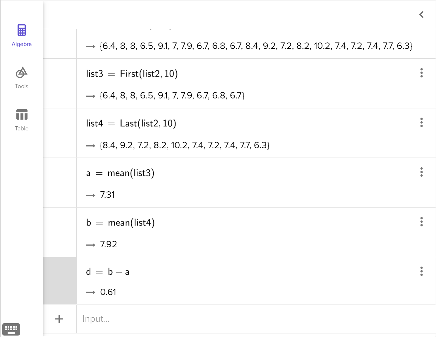
Control8.29.17.26.88.46.58.07.410.26.7
Treatment9.27.46.47.77.08.07.26.77.96.3
a

Determine the observed difference between the means of the two groups.

Worked Solution
Create a strategy

Find the mean of each group by using the formula: \text{Mean}=\dfrac{\text{Sum of the scores}}{\text{Number of scores}}. Then subtract the control group mean from the treatment group mean.

Apply the idea

Control group:

\displaystyle \text{Mean}\displaystyle =\displaystyle \dfrac{\text{Sum of the scores}}{\text{Number of scores}}Formula
\displaystyle =\displaystyle \dfrac{\text{8.2+9.1+7.2+6.8+8.4+6.5+8.0+7.4+10.2+6.7}}{\text{10}}Substitute in values
\displaystyle =\displaystyle 7.85Evaluate sum followed by division

Treatment group:

\displaystyle \text{Mean}\displaystyle =\displaystyle \dfrac{\text{Sum of the scores}}{\text{Number of scores}}Formula
\displaystyle =\displaystyle \dfrac{\text{9.2+7.4+6.4+7.7+7.0+8.0+7.2+6.7+7.9+6.3}}{\text{10}}Substitute in values
\displaystyle =\displaystyle 7.38Evaluate sum followed by division

Difference:

\displaystyle \text{Treatment mean} - \text{Control mean}\displaystyle =\displaystyle 7.38-7.85Difference of the two means
\displaystyle =\displaystyle -0.47Evaluate the subtraction
Reflect and check

The negative indicates the treatment group had a lower mean than the control group. We would be expecting this if the treatment was effective.

b

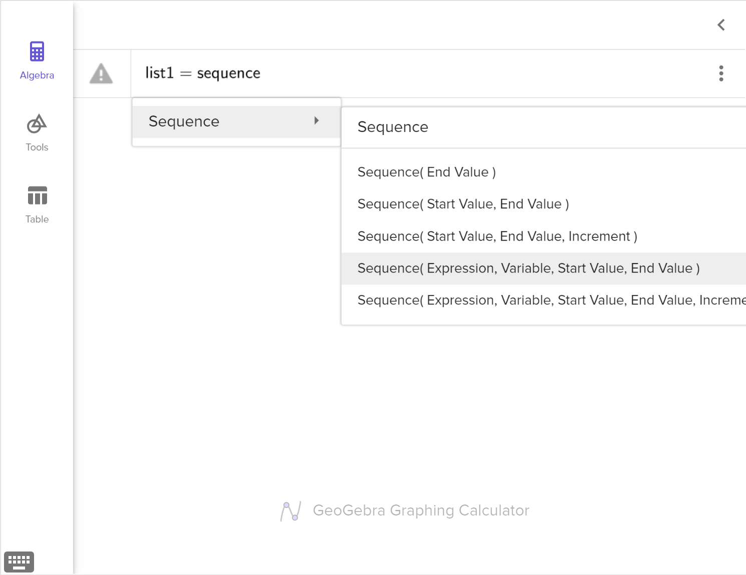
Randomly assign the data to two new groups and determine the difference of the means for this randomization.

Worked Solution
Create a strategy

We could write the numbers on pieces of paper and draw the pieces out of a hat randomly to form two new groups. Alternatively, we can use technology, such as a spreadsheet or Geogebra to randomize the sample.

Apply the idea

Example response of a randomization:

Using the Geogebra graphing calculator, we can enter the data as a single list.

A screenshot of the GeoGebra graphing calculator showing how to enter the following data as a list: 8.2, 9.1, 7.2, 6.8, 8.4, 6.5, 8.0, 7.4, 10.2, 6.7, ​9.2, 7.4, 6.4, 7.7, 7.0, 8.0, 7.2, 6.7, 7.9, 6.3. Speak to your teacher for more details.

We can then use the shuffle command to randomly rearrange the numbers in the list.

A screenshot of the GeoGebra graphing calculator showing how to use the Shuffle command to rearrange the following data in a list: 8.2, 9.1, 7.2, 6.8, 8.4, 6.5, 8.0, 7.4, 10.2, 6.7, ​9.2, 7.4, 6.4, 7.7, 7.0, 8.0, 7.2, 6.7, 7.9, 6.3. Speak to your teacher for more details.

Next, create two lists by using the commands First(list2, 10) and Last(list2, 10), to obtain the first and last 10 elements of list 2 respectively.

A screenshot of the GeoGebra graphing calculator showing how to split a list with 20 elements into two lists with 10 elements each. Speak to your teacher for more details.

Lastly, we can calculate the mean of each of our new lists and the difference.

A screenshot of the GeoGebra graphing calculator showing how to find the means of 2 new lists and the difference of their means. Speak to your teacher for more details.

The difference between the means of the two groups randomly assigned above is 0.61.

Reflect and check

How much did your simulation vary from the example create above? How much did the difference vary from the original group?

We could generate more samples by placing the cursor after the shuffle(list1) command and pressing enter. This will reshuffle and recalculate the commands below. We can record several simulations to create a sampling distribution of the difference of means using randomized groups.

c

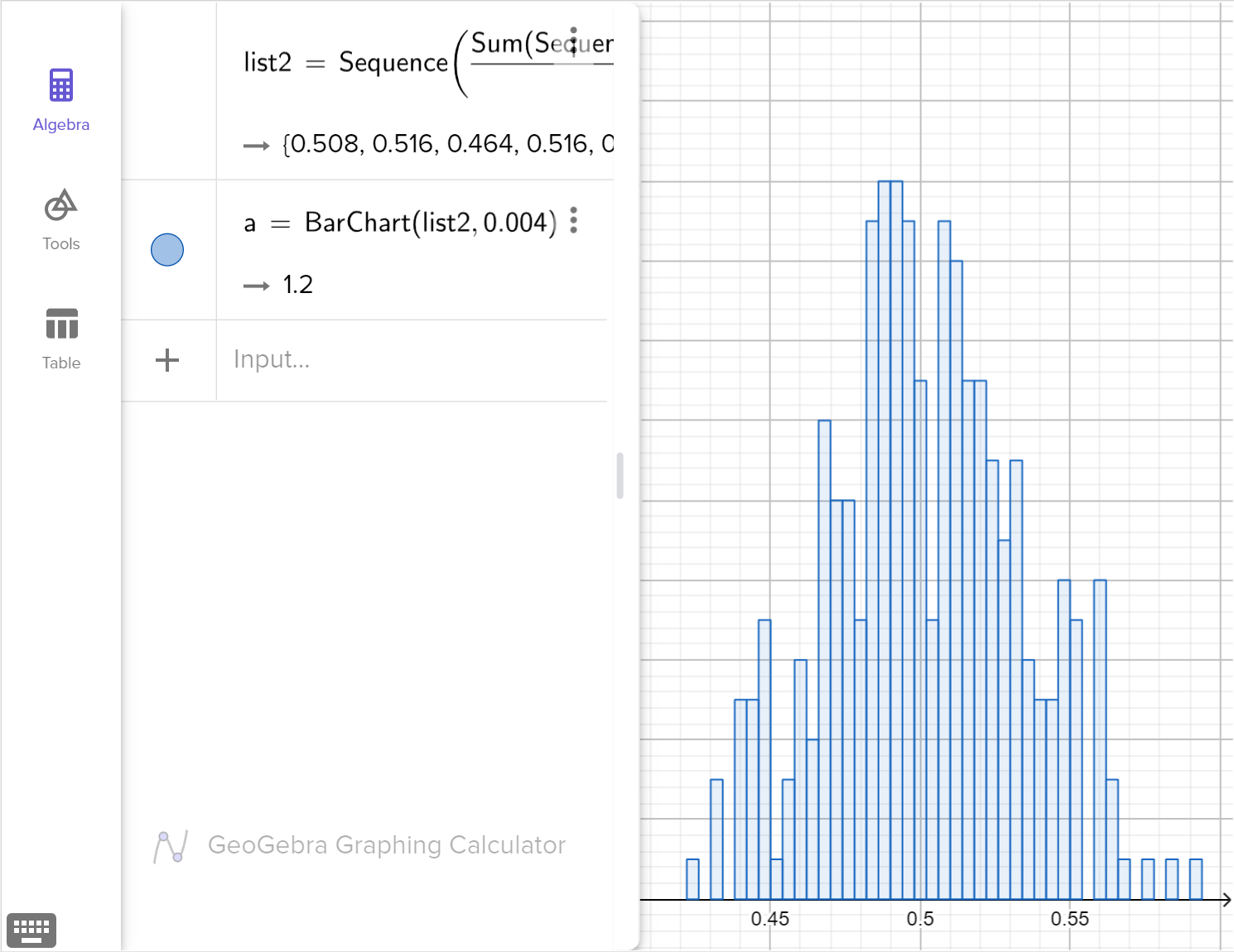
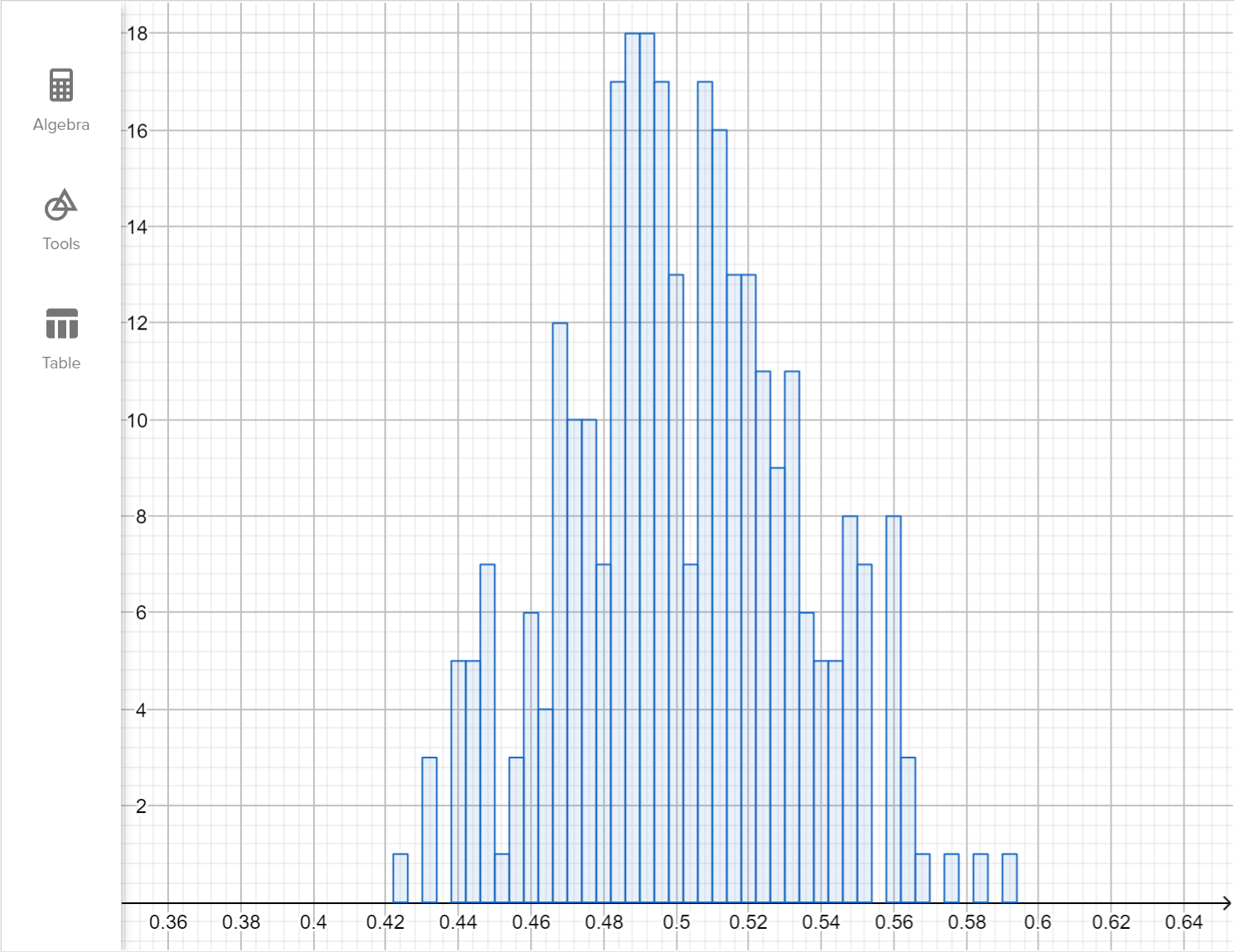
A sampling distribution for the difference of means using 200 random samples is shown below.

A histogram titled Difference of means using randomized groups with Frequency on the y-axis, with numbers 0 through 25, and Difference of group means on the x-axis, with bars labeled at their midpoint negative 1.5 to 1.8 in steps of 0.1. The negative 1.4 bar goes to 1 on the y-axis, negative 1.3 goes to 1, negative 1.1 goes to 2, negative 1 goes to 3, negative 0.9 goes to 4, negative 0.8 goes to 5, negative 0.7 goes to 3, negative 0.6 goes to 5, negative 0.5 goes to 7, negative 0.4 goes to 9, negative 0.3 goes to 11, negative 0.2 goes to 18, negative 0.1 goes to 16, 0 goes to 25, 0.1 goes to 12, 0.2 goes to 15, 0.3 goes to 21, 0.4 goes to 10, 0.5 goes to 6, 0.6 goes to 7, 0.7 goes to 5, 0.8 goes to 4, 0.9 goes to 4, 1 goes to 3, 1.2 goes to 1, 1.4 goes to 1, and 1.7 goes to 1.

Estimate the percentage of differences that were at or below the observed difference.

Worked Solution
Create a strategy

Count the outcomes that fall below the observed difference of -0.47 and state as a percentage out of the 200 samples shown.

Apply the idea

To estimate the number of outcomes at -0.47 or below, we can count the outcomes to the left of -0.45 on the histogram.

A histogram titled Difference of means using randomized groups with Frequency on the y-axis, with numbers 0 through 25, and Difference of group means on the x-axis, with bars labeled at their midpoint negative 1.5 to 1.8 in steps of 0.1. The negative 1.4 bar goes to 1 on the y-axis, negative 1.3 goes to 1, negative 1.1 goes to 2, negative 1 goes to 3, negative 0.9 goes to 4, negative 0.8 goes to 5, negative 0.7 goes to 3, negative 0.6 goes to 5, negative 0.5 goes to 7, negative 0.4 goes to 9, negative 0.3 goes to 11, negative 0.2 goes to 18, negative 0.1 goes to 16, 0 goes to 25, 0.1 goes to 12, 0.2 goes to 15, 0.3 goes to 21, 0.4 goes to 10, 0.5 goes to 6, 0.6 goes to 7, 0.7 goes to 5, 0.8 goes to 4, 0.9 goes to 4, 1 goes to 3, 1.2 goes to 1, 1.4 goes to 1, and 1.7 goes to 1. A red vertical dashed segment is between the negative 0.5 bar and negative 0.4 bar. The bars at the left of the red dashed line are marked red.

There are 31 outcomes less than -0.45. So approximately \dfrac{31}{200}=15.5\% of the differences would be at or below the observed difference.

Reflect and check

Alternatively, from the simulation we could find the mean and standard deviation of the sampling distribution created and use a table or technology to calculate the probability of a value being this extreme using a normal approximation of the distribution.

d

Explain whether or not the trial showed conclusively that the new medication is more effective than the current medication in improving how well the blood sugars were being controlled.

Worked Solution
Create a strategy

Using the percentage found in part (b) describe how likely it is that the observed difference occurred through natural variation.

Apply the idea

We found that 15.5\% of the differences would be at the observed level or below. This is not a particularly low value, indicating we would expect roughly 3 out of every 20 randomly selected samples could produce a negative difference at least as large as that observed in the trial. As there is a reasonable chance the observed difference occurred through natural variation, we cannot conclusively determine from the trial data that the new medication is more effective than the current medication.

Reflect and check

At what level would you consider the difference significant? Do you think this might vary depending on the application?

Example 2

A farmer runs a trial of a new diet for his chickens to test if it has any effect on the weight of the eggs produced. The farmer creates two small groups of hens, giving one group the new diet while keeping a control group on the current diet. He collects and weighs 20 eggs from each group. The eggs produced on the new diet had a mean weight of 59.8 \text{ g}, while the eggs on the original diet had a mean weight of 57.1 g.

The groups of chickens were then randomized and the difference in the mean weight recorded. The following distribution shows the results of 180 randomizations.

A histogram titled Difference of means using randomized groups with Frequency on the y-axis, with numbers 0 through 30, and Difference of group means on the x-axis, with bars labeled at their midpoint negative 3 to 3 in steps of 0.5. The negative 3 bar goes to 2 on the y-axis, negative 2.5 goes to 2, negative 2 goes to 11, negative 1.5 goes to 12, negative 1 goes to 23, negative 0.5 goes to 29, 0 goes to 24, 0.5 goes to 30, 1 goes to 16, 1.5 goes to 13, 2 goes to 7, 2.5 goes to 5, and 3 goes to 4.
a

Use the sampling distribution to determine whether or not the new diet makes a significant difference in increasing the weight of the eggs produced by the hens.

Worked Solution
Create a strategy

Find the difference in the mean of the control and treatment groups. Then, count the outcomes that fall above the observed difference in the sampling distribution and state as a percentage out of the 180 trials. Lastly, using the percentage found describe how likely it is that the observed difference occurred by chance.

Apply the idea

Difference in mean and control group:

\displaystyle \text{Difference}\displaystyle =\displaystyle \text{Treatment mean}-\text{Control mean}Formula
\displaystyle =\displaystyle 59.8- 57.1Substitute in values of means
\displaystyle =\displaystyle 2.7Evaluate the subtraction

To estimate the number of outcomes at 2.7 or above, we can count the outcomes to the right of 2.75 on the histogram.

A histogram titled Difference of means using randomized groups with Frequency on the y-axis, with numbers 0 through 30, and Difference of group means on the x-axis, with bars labeled at their midpoint negative 3 to 3 in steps of 0.5. The negative 3 bar goes to 2 on the y-axis, negative 2.5 goes to 2, negative 2 goes to 11, negative 1.5 goes to 12, negative 1 goes to 23, negative 0.5 goes to 29, 0 goes to 24, 0.5 goes to 30, 1 goes to 16, 1.5 goes to 13, 2 goes to 7, 2.5 goes to 5, and 3 goes to 4. A red vertical dashed segment is between the 2.5 bar and 3 bar. The 3 bar at the right of the red dashed line is marked red.

There are 4 outcomes greater than 2.75. So approximately \dfrac{4}{180}=2.2\% of the differences would be at or above the observed difference.

As the proportion is so low, there is a small chance that the observed difference occurred due to natural variation. We can conclude that the new diet increases the weight of the eggs produced.

Reflect and check

To then determine the size of the difference made by the new diet we could use the mean and sample standard deviation of the hens on the new diet to create an interval of likely values for the new average egg weight using a margin of error.

b

From the trial, determine if it would be reasonable to claim that the new diet increases the average weight of eggs by at least 2 grams, given that the sample of 20 eggs from hens on the new diet had a mean of 59.8g and a standard deviation of 3.6g and the eggs from hens on the original diet have a confirmed population mean weight of 57.1g.

Worked Solution
Create a strategy

We can use the margin of error to create a range of possible values we are confident the mean weight of eggs on the new diet lies within. Then we can look to see how far this interval lies from the mean of the eggs on the original diet.

Apply the idea

To determine a range of values for the improved mean on the new diet we can estimate the margin of error using: \text{Margin of error}\approx 2\dfrac{s}{\sqrt{n}}, where s is the sample standard deviation and n is the number of samples.

\displaystyle \text{Margin of error}\displaystyle \approx\displaystyle 2\dfrac{s}{\sqrt{n}}Formula
\displaystyle =\displaystyle 2\left(\dfrac{3.6}{\sqrt{20}}\right)Substitute s=3.6 and n=20
\displaystyle \approx\displaystyle 1.61Evaluate the division followed by the multiplication

Evaluating the sample mean of the new diet \pm the margin of error \left(59.8\pm 1.61\right), we find the range of likely values for the mean weight of the population of eggs from hens on the new diet.

We are confident that the mean weight of eggs for the new diet is between 58.19 and 61.41 grams.

In the worst case scenario, the mean weight of eggs for the new diet may be as low as 58.19 \text{ g}, which is only an improvement of 1.09 \text{ g} from the original mean weight of 57.1 \text{ g}.

In conclusion, while we are confident the new diet increases the weight of eggs produced, we cannot reasonably claim that the diet increases the average egg weight by at least 2 grams. Using the margin of error, the improvement may be as low as 1.09 grams.

Reflect and check

Instead of the simulation in part (a) we could use the margin of error alone to conclude the diet increases the mean weight. As the interval lies completely above the original mean of 57.1 \text{ g}, we could be confident the new mean is greater than the original. However, this would rely on accurately knowing the mean weight of eggs for the original diet.

Example 3

Otis works in a game store and claims that customers are more likely to be male. To support his claim, he records the gender of every tenth customer in the store over a week. At the end of the week he has recorded 135 males and 115 females enter the store.

Design a simulation to test whether or not the difference in the number of customers is significant enough to support Otis' claim.

Worked Solution
Create a strategy

If we assume the true proportion was in fact 50:50, how likely is it that 20 more males than females were observed out of a random sample of 250 customers? We want to simulate a trial with a 50:50 chance of males entering the store, and observe the range of proportions of 'males' out of 250 total customers that could result. We will need to repeat this trial multiple times to create a sampling distribution.

Apply the idea

We can simulate a coin being tossed using software by generating the numbers 0 or 1 randomly for 250 simulations. We can treat the 1's generated as male customers and the 0's generated as female customers.

To use Geogebra to generate random numbers, we can create a list and let it equal a sequence of numbers. Begin typing the word Sequence, and select the option for Sequence(Expression,Variable,Start Value,End Value).

A screenshot of the GeoGebra graphing calculator showing the five options for the Sequence command. The option Sequence left parenthesis Expression, Variable, Start Value, End Value right parenthesis is selected. Speak to your teacher for more details.

For the expression, we want it to generate random integers between 0 and 1, so we type the word Random and select RandomBetween(Minimum Integer, Maximum Integer).

A screenshot of the GeoGebra graphing calculator showing the two options for the RandomBetween command. The option RandomBetween left parenthesis Minimum Integer, Maximum Integer right parenthesis is selected. Speak to your teacher for more details.

Next, type 0 as the minimum integer, 1 as the maximum integer, and type a letter for the variable. To generate 250 numbers, the start value is 1 and the end value is 250.

A screenshot of the GeoGebra graphing calculator showing how to generate 250 random numbers, either 0 or 1, using the Sequence and RandomBetween commands. Speak to your teacher for more details.

Finally, we can find the proportion of male customers in the simulation by calculating the sum of the list divided by 250. This can be displayed as a fraction or a decimal by selecting \approx.

A screenshot of the GeoGebra graphing calculator showing how to find the average of a list of numbers. Speak to your teacher for more details.

By placing the cursor at the end of definition of list 1 and pressing enter, we can generate a new sample. Record the proportion for multiple trials to create a sampling distribution. Alternatively, we can generate a number of trials using technology and graph the trials in a histogram.

To generate 300 trials with 250 'customers' per trial, create a list with a sequence generating the proportion as the expression as shown in the screenshot.

A screenshot of the GeoGebra graphing calculator showing how to generate 300 random averages using the Sum, Sequence, and RandomBetween commands. Speak to your teacher for more details.

We can then create a bar chart of the results using the command BarChart(List of raw data, Width of bars, Vertical scale factor(optional)), with list2 as the raw data and 0.004 as the bar width.

A screenshot of the GeoGebra graphing calculator showing the following: on the left, a list of 300 random numbers between 0 to 1 using the Sum, Sequence, and RandomBetween commands and BarChart command using the list and on the right, a bar chart. Speak to your teacher for more details.

Zoom in to get an appropriate view window.

A screenshot of the GeoGebra graphing calculator showing a bar chart. Speak to your teacher for more details.

We can then count the outcomes that have a proportion greater than or equal to our observed proportion of \dfrac{135}{250}=0.54. In the simulation shown, there are 40 outcomes out of 300, which is 13\dfrac{1}{3}\%. So, while the observed number of customers does suggest more males shop at the store, the difference is not significant enough to confidently claim that this is the case. Our simulation shows that we would expect around 2 out of every 15 observations to show such a difference even if the true proportion was 50:50.

Reflect and check

To be confident in making such a claim Otis will need to observe a larger number of customers to reduce the chance that the outcome occurred due to natural variance. This is equivalent to reducing the margin of error for the sample proportion.

Idea summary

In an experiment, we often compare two groups. One is being given a treatment and the other is the control group without any treatment. We may observe statistical differences between the two groups. We need to decide if the differences are likely due to the treatment or to natural variation.

We can use simulation to shuffle the observed outcomes into two randomly assigned groups for a large number of trials. Then, we analyze the randomized sample distribution to determine how likely the observed statistical difference would occur due to natural variation.

This same randomization process can also be used in observational or survey studies, when we need to determine the likelihood that differences between two groups are due to chance, or if there may be some correlational relationship.

Outcomes

S.IC.B.5

Use data from a randomized experiment to compare two treatments; use simulations to decide if differences between parameters are significant.

S.IC.B.6

Evaluate reports based on data.

What is Mathspace

About Mathspace