
Introduction to a Normal Distribution
When the same measurement is made on a number of similar items, the recorded results constitute a data set of the kind referred to previously as univariate data.
For example, the amount of learning that has taken place in each student in a particular mathematics course might be measured by a formal test and the numerical results of the test are a univariate data set. Another example occurs when supposedly identical items are produced in a manufacturing process and measurements of a sample of the items are made to check that they are within specified tolerance limits. Generally, the measurements will vary around a mean value and if the process is working correctly will be not too far from the required value.
It often happens that most of the measurements will be clustered close to the mean value with the density of the observations falling off with distance away from the mean. Results of this kind displayed in a histogram show a central peak with columns of decreasing height on each side of the mean.
If there could be a vast number of observations put into the histogram with very narrow column widths, the variety of observations would give a bell-shaped histogram that reflects the way in which the frequencies of the observations diminish for values increasingly distant from the mean.
A data set that is symmetrical and bell-shaped about the mean, and which meets certain more precise shape requirements, is said to have a normal distribution or a normal probability density. It is an idealised notion since we can never have a sufficiently vast number of observations and narrow enough column widths to make the corresponding histogram. However, it is a useful mathematical model.
You may have heard of a bell curve, which is a colloquial term for a normally distributed set as this pattern occurs commonly. People's heights, IQ and weights are all roughly normally distributed. Two important values are needed to graph or interpret a normal distribution: the mean and the standard deviation. The mean ($\mu$μ) is the location of the maximum density of observations and is where the curve is highest. The curve is symmetrical about the mean. In fact, in a normally distributed data set, the mean, median and mode all take the same value.
The spread of the normal distribution will depend on its variance or the standard deviation $(\sigma)$(σ) which is the square root of the variance. This will affect how wide and how high the normal distribution is when graphed. The lower the standard deviation, the more clustered the scores will be around the mean. Conversely, the higher the standard deviation, the more spread the scores will be.
The average height of the distribution curve over a particular interval shows the proportion of observations expected to fall within that interval. If the variance is low, the proportion of observations near the mean will be high and the curve will be high at the mean value. If the variance is high, the proportion of observations near the mean is reduced and therefore the curve is not so high at the mean.
For example, this distribution curve comes from a data set that has a very small standard deviation, $\sigma=0.2$σ=0.2, and hence is clustered tightly around the mean:

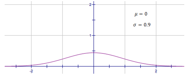
whereas this normal distribution has a larger standard deviation, $\sigma=0.9$σ=0.9, and hence is quite spread.
To see how a change in the mean and standard deviation affects the shape of the normal distribution curve, check out this graph. By moving the sliders around you can vary the mean and standard deviation, and see how the bell curve changes as a result.
Worked Examples
QUESTION 1
Which of the following sets of data is approximately normally distributed?
- ABC
QUESTION 2
Which two of the following statements are true for a normal distribution curve?
There are the same number of scores above and below the mean.
AThe curve is symmetrical.
BThe fewest scores lie around the mean.
CThe curve is asymmetrical.
D
QUESTION 3
A sample of professional basketball players is normally distributed and gives the mean height as $199$199 cm with a standard deviation of $10$10 cm.
How tall is a basketball player who is $3$3 standard deviations above the mean?
How tall is a basketball player who is $1.5$1.5 standard deviations below the mean?