
When we have a set of univariate data, it often happens that most of the measurements will be clustered close to the mean value with the density of the observations falling off as distance away from the mean increases. Results of this kind displayed in a histogram show a central peak with columns of decreasing height on each side of the mean.
The normal distribution is a special type of continuous probability distribution. It is often called the "bell curve" because of the shape of the graph. The normal distribution is important in statistics because it can be used to describe many natural variables. For example, a person's height versus arm span, and IQ are both examples of normal distributions.
The bell curve is symmetrical about the mean (which is the top of the bell) and it has the property that the mean, mode and median are all equal.
Probability distributions that display bell curve properties are described as being "normally distributed".

The shape of the normal distribution will depend on its mean ($\mu$μ) and standard deviation $(\sigma)$(σ). The mean is where the graph peaks. To draw normal distribution graph we only need the mean and standard deviation values.
For the normal distribution, the mean is exactly in the middle, so $50%$50% of the values are above the mean and $50%$50% of the values are below the mean.
Almost all of the scores lie within $3$3 standard deviations either side of the mean.
The lower the standard deviation, the more clustered the scores will be around the mean. Conversely, the higher the standard deviation, the more spread the scores will be.
For example, this distribution curve comes from a data set that has a very small standard deviation of $\sigma=0.2$σ=0.2, and as such the scores are clustered tightly around the mean:

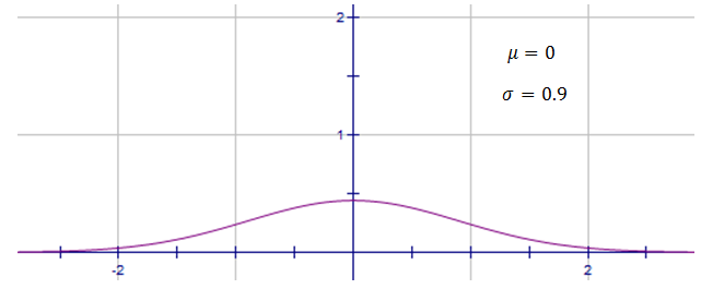
This normal distribution, on the other hand, has a larger standard deviation of $\sigma=0.9$σ=0.9. Its scores are much more spread out.
To see how a change in the mean and standard deviation affects the shape of the normal distribution curve, check out the applet below. By moving the sliders around you can vary the mean and standard deviation, and see how the bell curve changes as a result.
Practice questions
QUESTION 1
Which of the following sets of data is approximately normally distributed?
- ABC
QUESTION 2
Which two of the following statements are true for a normal distribution curve?
There are the same number of scores above and below the mean.
AThe curve is symmetrical.
BThe fewest scores lie around the mean.
CThe curve is asymmetrical.
D
QUESTION 3
A sample of professional basketball players is normally distributed and gives the mean height as $199$199 cm with a standard deviation of $10$10 cm.
How tall is a basketball player who is $3$3 standard deviations above the mean?
How tall is a basketball player who is $1.5$1.5 standard deviations below the mean?
The normal distribution formula
The probability density function describing the normal distribution function is written in terms of the mean ($\mu$μ) and standard deviation ($\sigma$σ):
$\phi\left(x\right)=\frac{1}{\sigma\sqrt{2\pi}}e^{-\frac{\left(x-\mu\right)^2}{2\sigma^2}}$ϕ(x)=1σ√2πe−(x−μ)22σ2
We won't be using this formula to find the probabilities. Instead, we will be using a table of values in a later lesson.
Exploration
Assume that a population is normally distributed with mean $\mu=a$μ=a and standard deviation $\sigma=b$σ=b. Use graphing software to sketch the graph of $\phi\left(x\right)$ϕ(x), adding sliders for $a$a and $b$b to explore the effects of changing the mean and standard deviation on the bell curve.
- What do you notice about the graph?
- What happens when $b$b gets close to $0$0?