
Organising data: frequency distribution table
After we have collected our data, the information needs to be organised before we can analyse it. A frequency distribution table is a useful way to do this for both categorical and numerical data as it shows the number of times each different event or result occurred.
Categorical data example
As an example, let's say the colour of every car that passed through a given intersection was recorded over a ten minute period:
green, white, yellow, white, black, green, black, blue, blue, silver, white, black, green, blue, blue, white, black, silver, silver, red, red, red, black, white, blue, white, black, silver, silver, white, blue, white, black, yellow, blue, white, white, red, green, silver, black, white, black, white.
We can see that the same colours are occurring multiple times, so it makes sense to organise the data using a frequency table. If the data is categorical, the table can be used to create a bar chart.
|
 |
Notice that the frequency table has three columns:
- The first column shows the subgroups within the data
- The tally column (optional) uses tally marks to record the frequency of each subgroup
- The final column sums the tally marks and records the frequency as a number
Not all frequency tables contain a tally column but it can make it easier to count the number of occurrences correctly.
The sum of the frequencies is equal to the total number of data values. In this case, the colours of $44$44 vehicles were recorded.
Numerical data example
In the example below, a person who exercises most days has recorded the time to the nearest minute they spend on daily exercise over an entire year. The data is first organised into a frequency table.
|
 |
For numerical data like this, a frequency histogram is used instead of a bar graph. This will be explained more below.
When data is organised in a frequency distribution table it makes it easier to find the mean, median, mode and range. For the mean, we can add a column called the "$f$f$\times$×$x$x" column to help us find the mean. Alternatively, the mean from a frequency distribution table can also be found by using the statistics mode on your calculator.
Practice question
Question 1
A statistician organised a set of data into the frequency table shown:
Complete the frequency distribution table:
Score ($x$x) Frequency ($f$f) $f\times x$f×x $31$31 $12$12 $\editable{}$ $32$32 $14$14 $\editable{}$ $33$33 $7$7 $\editable{}$ $34$34 $20$20 $\editable{}$ $35$35 $15$15 $\editable{}$ Totals $\editable{}$ $\editable{}$ Calculate the mean, correct to two decimal places.
Find the range of the scores in the table above.
Find the mode of the set of scores in the table.
Displaying data
There are various graph types to choose from to display the data you have collected. The type of graph will depend on the type of data you have and the purpose of the investigation.
The graphs we will focus on in this lesson to display data are:
- Divided bar graphs
- Bar and column graphs
- Sector graphs (or pie charts)
- Dot plots
- Stem and leaf plots
- Frequency histograms
- Frequency polygons
- Line graphs
For categorical data, the most appropriate graphs will be the divided bar graph, bar and column graphs, sector graphs, dot plots, two-way tables and Pareto charts. The latter two graphs will be studied in a later lesson.
For numerical data, we can use dot plots, stem and leaf, frequency histograms, frequency polygons and line graphs.
When data is organised and graphed it can make it easier to analyse.
Pie charts (sector graphs)
Pie charts are also called sector graphs because the pieces of the pie are mathematically referred to as sectors. The total circle represents all the scores in a data set. Since the angle in the circle is $360^\circ$360°, each category's frequency is a proportion of $360^\circ$360°.
Practice question
Question 2
The sector graph represents the number of people taking leave from work at a particular company.

If $5$5 people took leave in January, how many degrees represent $1$1 person?
How many people took leave in November?
How many people took leave between the beginning of November and the end of March?
What percentage of the people took leave in December?
Give your answer as a percentage, rounding to two decimal places.
Divided bar graphs
A divided bar graph is a rectangle (or bar) that is split up into different sections like this:

The size of each section represents the proportion or fraction of the whole amount that is being graphed. We can see in the graph above that hockey is the least popular sport, as it takes up the smallest part of the bar. Conversely, soccer is the most popular sport as it takes up the biggest amount of the bar.
Bar graphs
Bar graph is a generic name for any graph that displays information using rectangular or cylindrical bars.
Worked example
Example 1
The sales of different products are shown in the following bar graph.

a) Which is the best-selling product?
Think: The best-selling product will have the longest line in the bar graph.
Do: Product D is the best-selling product.
b) How many units of all products were sold in total?
Think: We need to add the frequency of each column. Remember that each value is multiplied by $1000$1000.
Do: $9000+6000+5000+10000+9000+7000=46000$9000+6000+5000+10000+9000+7000=46000 units
Column graphs
A column graph is the name for a specific type of bar graph that uses vertical bars, so they appear like columns. Column graphs are used to show categories of data that you have counted. In a column graph, the height of the column shows the number of scores. Both the horizontal and vertical axes should be labelled to help explain the information in the graph.
Practice question
Question 3
A survey of the preferred sport was done for a group of boys and the results are shown in the bar graph below:
How many boys prefer football to other sports?
Which is the most popular sport?
Football
ATennis
BRugby
CBasketball
DHockey
EHow many boys took part in the survey?
Frequency histograms
Although a histogram looks similar to a bar chart, there are a number of important differences between them:
- Histograms show the distribution of data values, whereas a bar chart is used to compare data values.
- Histograms are used for numerical data, whereas bar charts are often used for categorical data.
- A histogram has a numerical scale on both axes, while a bar chart only has a numerical scale on the vertical axis.
- The columns in a bar chart could be re-ordered, without affecting the representation of the data. In a histogram, each column corresponds with a range of values on a continuous scale, so the columns cannot be re-ordered.
 |
 |
|
| Histogram | Bar chart |
Key features of a frequency histogram:
- The horizontal axis is a continuous numerical scale (like a number line). It represents numerical data, such as time, height, mass or temperature, and may be divided into class intervals.
- The vertical axis is the frequency of each data value or class interval.
- There are no gaps between the columns because the horizontal axis is a continuous scale. It is possible for a class interval to have a frequency of zero, but this is not the same as having gaps between each column.
- It is good practice, when creating a histogram, to leave a half-column-width gap between the vertical axis and the first column.
Note: Frequency histograms and polygons are usually for numerical continuous data however you may be asked to draw these for numerical discrete data as well.
Practice question
Question 4
The amount of snowfall (in centimetres) is recorded at the base of the mountain each day.
To create a frequency histogram of the data, which values go on the horizontal axis?
Number of days it snowed each amount
AAmount of snowfall
BThe snowfall recorded each day, to the nearest centimetre, is as follows:
$6,2,0,3,2,2,3,4,2,0,3,2,3,4,6,4,3,0,5,3$6,2,0,3,2,2,3,4,2,0,3,2,3,4,6,4,3,0,5,3
Construct a frequency histogram of the data.
On how many days did $3$3 centimetres of snow fall?
On how many days did at least $4$4 centimetres of snow fall?
Frequency polygons
Frequency polygons are particularly useful for helping us understand the shapes of distributions and for comparing data sets.
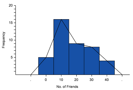
- A frequency polygon is drawn by joining the middle-top points of the columns of a histogram, as shown below.
- The line starts and ends on the horizontal axis half a column width to the left and right of the first and last column respectively.
- A frequency polygon is suitable for numerical continuous data and can be drawn together with a histogram or by itself.
-
If we look at the way the frequency polygon 'cuts off' triangles from the columns of the histogram, we can see that the area under the frequency polygon is equal to the area of the columns.
 '
'
We can use frequency polygons to help us estimate how many people got a particular score. For example, the graph above indicates that $6$6 people have $35$35 friends.
Practice question
Question 5
Some people were asked approximately how many of their high school friends they remained in contact with after high school. Each approximated to the nearest 10 friends. The results are presented in the frequency distribution table:
| Score | Frequency |
|---|---|
| $0$0 | $5$5 |
| $10$10 | $16$16 |
| $20$20 | $9$9 |
| $30$30 | $8$8 |
| $40$40 | $4$4 |
Construct a frequency histogram for the data.
What was the most common response?
A frequency polygon is added to the histogram.
Using the polygon, estimate the number of people who kept in touch with $35$35 friends.
$3$3
A$9$9
B$6$6
CWhich of the following is true? A frequency polygon:
only allows you to determine the frequency of each known score
Aallows you to determine the frequency of any score with certainty
B
Line graphs
Line graphs are used to display continuous data and are often used to show changing information over time. Examples of data that could be displayed in a line graph include temperature, your heart rate throughout the day and a company's daily sales.
Basically, a line graph is drawn as one continuous line to show a continual (usually changing) set of scores.
Worked example
Example 2
The line graph below shows how the temperature changed throughout the day.

a) What was the temperature at $6$6am?
Think: Let's find $6$6am on the horizontal axis, then look up to the red line, then to the corresponding point on the vertical axis.
Do: It was $15^\circ$15°C at $6$6am.
b) At what time was the temperature the hottest?
Think: When does the red line reach the highest point?
Do: It is hottest at $2$2pm.
Dot plots
Dot plots are a graphical way of displaying the distribution of numerical or categorical data on a simple scale with dots representing the frequency of outcomes. They are best used for small to medium size sets of data and are good for visually highlighting how the data is spread and whether there are any gaps in the data or outliers.
In a dot plot, each individual data value is represented by a single dot, displayed above a horizontal line. When data values are identical, the dots are stacked vertically. The graph appears similar to a column graph with the number of dots representing the total count.

- To correctly display the distribution of the data, the dots must be evenly spaced in columns above the line
- The scale or categories on the horizontal line should be evenly spaced
- A dot plot does not have a vertical axis
- The dot plot should be appropriately labelled
Practice question
Question 6
The goals scored by a football team in their matches are represented in the following dot plot.

Complete the following frequency distribution table.
Goals scored Frequency $0$0 $\editable{}$ $1$1 $\editable{}$ $2$2 $\editable{}$ $3$3 $\editable{}$ $4$4 $\editable{}$ $5$5 $\editable{}$
Stem and leaf plot
A stem and leaf plot, or stem plot, is used for organising and displaying numerical data. It is appropriate for small to moderately sized data sets.
In a stem and leaf plot, the units digit in each data value is split from the other digits, to become the 'leaf'. The remaining digits become the 'stem'.
The values in a stem and leaf plot are generally arranged in ascending order (from lowest to highest) from the centre out. This is called an ordered stem and leaf plot.
The data values $10,13,16,21,26,27,28,35,35,36,41,41,45,46,49,50,53,56,58$10,13,16,21,26,27,28,35,35,36,41,41,45,46,49,50,53,56,58 are displayed in the stem and leaf plot below.

- The stems are arranged in ascending order, to form a column, with the lowest value at the top
- The leaf values are arranged in ascending order from the stem out, in rows, next to their corresponding stem
- There are no commas or other symbols between the leaves, only a space between them
 |
 |
Practice question
Question 7
The stem-and-leaf plot below shows the age of people to enter through the gates of a concert in the first $5$5 seconds.
| Stem | Leaf | |
| $1$1 | $1$1 $2$2 $4$4 $5$5 $6$6 $6$6 $7$7 $9$9 $9$9 | |
| $2$2 | $2$2 $3$3 $5$5 $5$5 $7$7 | |
| $3$3 | $1$1 $3$3 $8$8 $9$9 | |
| $4$4 | ||
| $5$5 | $8$8 | |
|
||
How many people passed through the gates in the first $5$5 seconds?
What was the age of the youngest person?
The youngest person was $\editable{}$ years old.
What was the age of the oldest person?
The oldest person was $\editable{}$ years old.
What proportion of the concert-goers were under $20$20 years old?
Describing the distribution of data from a graph
When we describe the shape of data sets, we want to focus on how the scores are distributed and whether the shape is symmetrical or not.
Symmetry
Data may be described as symmetrical or asymmetrical.
There are many cases where the data tends to be around a central value with no bias left or right. In such a case, roughly $50%$50% of scores will be above the mean and $50%$50% of scores will be below the mean. A well known symmetrical distribution is the normal distribution which is often described as a "bell-shaped curve".
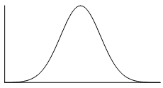
The picture below shows how the normal distribution can occur on a histogram. The dark line shows the nice, symmetrical curve that can be drawn over the histogram.

In the distribution below, the $0$0 point in the middle represents the mean, the median and the mode - all these measures of central tendency are equal for this distribution since it is symmetrical. If we use the line at $0$0 as our axis of symmetry, notice that the left-hand side is a perfect reflection of the right-hand side.

Skewness
If a data set is asymmetrical instead (i.e. it isn't symmetrical), it may be described as positively or negatively skewed.
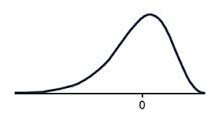
Positive skew
A data set that has positive skew has a long tail of values above the peak of the graph, such that more than half of the scores are above the peak. This means the mean is greater than the median, which is greater than the mode.
MODE < MEDIAN < MEAN
A positively skewed graph looks something like this.
Notice that there are more scores above the peak than below the peak.
Negative skew
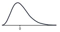
A data set that has negative skew (sometimes called a 'left skew') has a long tail of values below the peak of the graph, such that more than half of the scores are below the peak. This means the mode is greater than the median, which is greater than the mean.
MEAN < MEDIAN < MODE
A negatively skewed graph looks something like this.
Notice that there are more scores below the peak than above the peak.
Clustering and gaps
In a set of data, a cluster occurs when a large number of the scores are grouped together within a very small range. Gaps can occur when there are in-between scores that have no frequency.
Outliers
The shape of the data also shows us whether there are any outliers or unusually high or low scores in our data set.
For example, in the dot plot below, do you see how all the scores range between $12$12 and $14$14 except one? This means that $24$24 is an outlier.

In this case, the score is very obviously far outside the range of the rest of the data set.
Modality
Modality describes the prevalence of local peaks in a data set. The peaks don't necessarily need to be the mode of the whole data set, but rather a local cluster of data that is more frequent and stands out from the surrounding data. When we look at the modality of a data set, it is usually useful to examine a graph of the data.
We describe modality by the number of peaks. A data set that has two distinct peaks, like in the frequency polygon below, is called bimodal.

To determine the modality of a distribution, we can simply identify the number of modal peaks. For instance, we would say that the data shown in the dot plot below has three modal peaks because there are local peaks at scores of $6$6, $12$12, and $20$20.

Practice questions
Question 8
How many peaks are there on the graph?

$\editable{}$ peaks
Question 9
State whether the scores in each histogram are positively skewed, negatively skewed or symmetrical (approximately).
A histogram that represents the distribution of scores. The x-axis enumerates discrete scores as individual points, while the y-axis corresponds to the frequency of each score interval. Each bar on the histogram corresponds to one of these distinct scores, with the bar's height reflecting the count or frequency of occurrences for that particular score. Most of the scores are relatively high. Positively skewed
ASymmetrical
BNegatively skewed
CA histogram that represents the distribution of scores. The x-axis enumerates discrete scores as individual points, while the y-axis corresponds to the frequency of each score interval. Each bar on the histogram corresponds to one of these distinct scores, with the bar's height reflecting the count or frequency of occurrences for that particular score. Approximately, as the score goes higher, the frequency goes lower. Positively skewed
ANegatively skewed
BSymmetrical
CA histogram that represents the distribution of scores. The x-axis enumerates discrete scores as individual points, while the y-axis corresponds to the frequency of each score interval. Each bar on the histogram corresponds to one of these distinct scores, with the bar's height reflecting the count or frequency of occurrences for that particular score. The scores have its peak approximately in the middle. Negatively skewed
ASymmetrical
BPositively skewed
C
Question 10
For the Stem and Leaf plot attached:
| Stem | Leaf | |
| $0$0 | $5$5 | |
| $1$1 | $7$7 $8$8 | |
| $2$2 | $0$0 $8$8 | |
| $3$3 | $0$0 $4$4 $6$6 $7$7 $8$8 $9$9 | |
| $4$4 | $1$1 $3$3 $5$5 $8$8 $8$8 $8$8 | |
| $5$5 | ||
| $6$6 | ||
| $7$7 | ||
| $8$8 | ||
| $9$9 | $3$3 | |
|
||
Are there any outliers?
Yes
ANo
BIdentify the outlier.
Is there any clustering of data?
Yes
ANo
BWhere does the clustering occur?
10s - 20s
A30s - 40s
B20s - 30s
CWhat is the modal class(es)?
10-19
A40-49
B30-39
C20-29
DNot including the outlier, the distribution of the data is:
Positively skewed
ASymmetrical
BNegatively skewed
C