
We look for a model that will summarise an apparent relation between two variable quantities. The model, if successful, will enable predictions to be made about further observations of an experiment and it may help in developing an understanding of the mechanisms involved in a process.
As a rule, we look for the simplest model that will provide a reasonably good fit for a set of data. And, of all possible models, a linear model is the simplest.
Even when it is clear that a nonlinear model would describe the data better than would a linear model, we may choose to use a linear model that will be approximately correct over a small portion of the data range. We may wish to approximate a complicated nonlinear process by a string of separate linear models that each apply to a small sub-range of the data.
Example 1
At most coastal locations in New South Wales, and elsewhere. the tides are observed to have a period of approximately $8$8 hours. Suppose measurements of the water level at a particular place are taken every $2$2 hours over a span of one day. The results are displayed in the following plot.
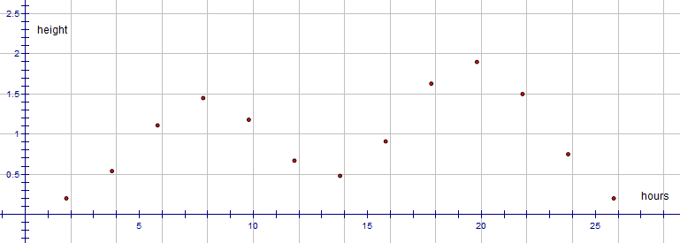
There is a repeating pattern which could be modelled using sine or cosine functions but, as an approximation, we could fit several straight lines, each applicable to a part of the range.

We must be careful with modelling in this way to specify which linear graph is applicable for each part of the range of data. For example, the left-most line applies to the time period from about $2$2 hours to $8$8 hours, and so on.
The choice of a mathematical model for data often rests on extra information or assumptions about the data. For example, the idea of modelling the tide data using trigonometric functions comes from considerations beyond the actual data. We believe, before any data is collected, that the tides follow a repeating pattern. Therefore, we will need a mathematical function that repeats. Combinations of the sine function have this property.
If we did not use extra knowledge or common sense of this sort we might try modelling the tidal data using a polynomial function. One might find by experiment that it is possible to discover a degree $6$6 polynomial that fits the collected data very closely. However, just as with the linear approximations, we would have to specify that the function only applies in the particular $24$24-hour time period. This polynomial model would be wildly inaccurate on subsequent days because the polynomial increases without bound outside of the small window of time in which the data set was obtained.
Example 2
It is proposed to carry out an experiment to do with trees that are being grown for timber in a plantation. The researchers are interested in the diameters of the tree trunks at time intervals after the trees were first planted. Before any measurements are made, various theories are discussed concerning the possible outcomes.
On the basis of this thinking, certain mathematical models are discarded as being impossible or unlikely and the experiment proceeds with the aim of discovering which of the remaining, plausible models seems to best reflect reality.
- The model would have to be an increasing function, at least up to some point, because the trees will never reduce in size.
- The rate of increase might decline with time because the available nutrients the tree needs for growth are going into increasing the height of the tree as well as the diameter.
- The rate of increase in diameter might decrease because this will still allow the cross-sectional area of a tree trunk to increase at a steady rate.
- The rate of increase in the diameter might stay fairly constant because the tree is developing a stronger root system to maintain its nutrient supply and its growth rate.
- The pattern of growth might be erratic and somewhat unpredictable because of variations in climate.
On the basis of this thinking, the researchers would probably discard an exponential model, a quadratic model, all periodic functions and various others, but might consider linear models (including composites of several linear pieces), a logarithm function, a square root function, or one of the several special S-shaped functions.
Worked Examples
Question 1
Every week, Rochelle deposits $\$800$$800 into a savings account. She plots her accumulated savings over several weeks.
Would a linear model accurately describe Rochelle’s savings after the first week? Choose the most appropriate response.
No, Rochelle's savings will not change over time.
AYes, the difference in the balance from week to week increases at a linear rate.
BYes, the accumulated savings will approach a constant amount after many weeks.
CYes, for every week that passes, Rochelle's savings will increase by a constant amount.
D
Question 2
Due to a certain process of nuclear decay, the amount of Potassium-40 in a geological sample halves every $0.13$0.13 billion years. The scatter plot below compares the age of a sample ($t$t, in billions of years) with the proportion ($P$P) of the original amount of Potassium-40 present in the sample, for several different geological samples. The graph also features an exponential model.
As $t$t gets larger and larger, what value does $P$P approach?
The value of $P$P will approach $\editable{}$.
Consider a particular geological sample containing an initial amount of Potassium-40. As this sample ages, will the amount of Potassium-40 present always be greater than zero?
Yes, the amount present will continue to halve every $0.13$0.13 billion years and never reach zero.
ANo, there will ultimately be no Potassium-40 left in the sample.
B
Question 3
A supermarket uses rectangular prism cardboard boxes of different widths, $x$x, and volumes, $y$y. A scatter plot of different sized boxes is shown below.
Jack is an employee who usually packs and unpacks smaller boxes. He uses the following linear model to represent the box sizes:
Loading Graph...A scatterplot is shown on a Cartesian plane with the x-axis ranging from $20$20 to $50$50 labeled in major intervals of 5 and minor intervals of 1, and the y-axis ranging from $4500$4500 to $8500$8500 labeled in major intervals of 500 and minor intervals of 1. The data points plotted are at $\left(24,4794\right)$(24,4794), $\left(26,5396\right)$(26,5396), $\left(28,5782\right)$(28,5782), $\left(30,6000\right)$(30,6000), $\left(35,6125\right)$(35,6125), $\left(40,6250\right)$(40,6250), $\left(42,6468\right)$(42,6468), $\left(44,6854\right)$(44,6854), and $\left(46,7456\right)$(46,7456). The coordinates of the data points are not explicitly labeled. A straight line passing through points $\left(24,4794\right)$(24,4794) and $\left(30,6000\right)$(30,6000) is drawn. For which values of $x$x is this model most accurate?
$30\le x\le40$30≤x≤40
A$40\le x\le46$40≤x≤46
B$24\le x\le46$24≤x≤46
C$24\le x\le30$24≤x≤30
DGeorgia is an employee who usually packs and unpacks larger boxes. She uses a different linear model to represent the box sizes, shown below:
Loading Graph...A scatterplot is shown on a Cartesian plane with the x-axis ranging from $20$20 to $50$50 labeled in major intervals of 5 and minor intervals of 1, and the y-axis ranging from $4500$4500 to $8500$8500 labeled in major intervals of 500 and minor intervals of 1. The data points plotted are at $\left(24,4794\right)$(24,4794), $\left(26,5396\right)$(26,5396), $\left(28,5782\right)$(28,5782), $\left(30,6000\right)$(30,6000), $\left(35,6125\right)$(35,6125), $\left(40,6250\right)$(40,6250), $\left(42,6468\right)$(42,6468), $\left(44,6854\right)$(44,6854), and $\left(46,7456\right)$(46,7456). The coordinates of the data points are not explicitly labeled. A straight line passing through points $\left(40,6250\right)$(40,6250) and $\left(46,7456\right)$(46,7456) is drawn. For which values of $x$x is this model most accurate?
$40\le x\le46$40≤x≤46
A$24\le x\le46$24≤x≤46
B$30\le x\le40$30≤x≤40
C$24\le x\le30$24≤x≤30
DThe graph below shows both Jack's and Georgia's models for the values of $x$x that they most accurately describe:
Loading Graph...A scatterplot is shown on a Cartesian plane with the x-axis ranging from $20$20 to $50$50 labeled in major intervals of 5 and minor intervals of 1, and the y-axis ranging from $4500$4500 to $8500$8500 labeled in major intervals of 500 and minor intervals of 1. The data points plotted are at $\left(24,4794\right)$(24,4794), $\left(26,5396\right)$(26,5396), $\left(28,5782\right)$(28,5782), $\left(30,6000\right)$(30,6000), $\left(35,6125\right)$(35,6125), $\left(40,6250\right)$(40,6250), $\left(42,6468\right)$(42,6468), $\left(44,6854\right)$(44,6854), and $\left(46,7456\right)$(46,7456). The Two line segments connecting $\left(24,4794\right)$(24,4794) to $\left(30,6000\right)$(30,6000) and $\left(40,6250\right)$(40,6250) to $\left(46,7456\right)$(46,7456) are drawn. The coordinates of the data points are not explicitly labeled or given. Points $\left(24,4794\right)$(24,4794), $\left(26,5396\right)$(26,5396), $\left(28,5782\right)$(28,5782) and $\left(30,6000\right)$(30,6000) are relatively close to the line representing Jack's model. Points $\left(40,6250\right)$(40,6250), $\left(42,6468\right)$(42,6468), $\left(44,6854\right)$(44,6854) and $\left(46,7456\right)$(46,7456) are relatively close to the line representing Georgia's model. Do the two models together accurately describe all of the boxes used by the supermarket? Choose the most appropriate response.
Yes - Jack's model describes all of the small boxes, and Georgia's model describes all of the large boxes, so together they must describe all of the boxes.
ANo - There are boxes used by the supermarket with $x>46$x>46 that are not described accurately by either model.
BYes - Jack's model is accurate in the region $24\le x\le30$24≤x≤30 and Georgia's model is accurate in the region $40\le x\le46$40≤x≤46, and together these are all the possible values for $x$x.
CNo - Jack's model is only accurate in the region $24\le x\le30$24≤x≤30 and Georgia's model is only accurate in the region $40\le x\le46$40≤x≤46, but there is a box used by the supermarket that has $x=35$x=35 which is in neither region.
D