topic badge

6.07 Modeling with rational functions (M)

Introduction

In lesson  4.04 Modeling with polynomial functions  , we focused on the first part of the modeling process: identifying the problem and creating and analyzing the model. Now, while modeling rational functions with real-world phenomena, we will focus on the second half of the modeling process: interpreting results and revising the model.

A modeling cycle. Starting with the phrase Identify the problem inside a circle. An arrow pointing to the right where the phrase Create a model is inside a rectangle. Next is an arrow pointing downward where the phrase Apply and analyze is inside a rectangle. Then, an arrow pointing to the right where the phrase Interpret results is inside a rectangle. Next is an arrow pointing upward where the phrase Verify the model is inside a triangle. Then, an arrow pointing to the right where the phrase Report findings is inside a circle. There is an arrow pointing to the left from the phrase Verify the model to Create a model.

Interpreting results, drawing conclusions, and revising models

After a problem has been identified, the model is created. Then, we apply the model and analyze it for accuracy and effectiveness. We interpret the results that come from the use of the model and draw any relevant conclusions to the context.

Interpreting results includes the following:

  • Determining whether the answer makes sense in terms of the context

  • Identifying any extraneous solutions from the model that don't apply to the situation

  • Discussing the potential accuracy of the model depending on the limitations of the model or the assumptions we made when creating the model

At some point during analyzing or interpreting the model, we may realize the model needs to be revised. There are several different reasons a model might need to be modified. Here are some examples:

There might be an error in calculations, assumptions, or use of units.

We may have new or more relevant information to work with, requiring adjustments.

Sometimes our model needs fixing because we didn't consider all the consequences of making certain choices. For example, a problem involving a range of rates requires some choices to be made about what rate to use in that range. After analyzing the model, we may decide to choose a different rate analysis, not because of new information or an error, but because we realize a different choice would provide better information or be more relevant to the problem situation.

In other cases, our model may be too limited and need to be revised to account for broader considerations.

Examples

Example 1

200 \text{ gallons} of water are mixed in a 500-gallon aquarium with 22.5 cups of reef salt. A hose, when turned on, will add water at a rate of 5 \text{ gal/min} while salt is poured in at a rate of 120 \text{ c/hr}.

An aquarium being filled with water through a hose.

Note that the safety of salinity for a saltwater aquarium is between 1 \% and 3 \%.

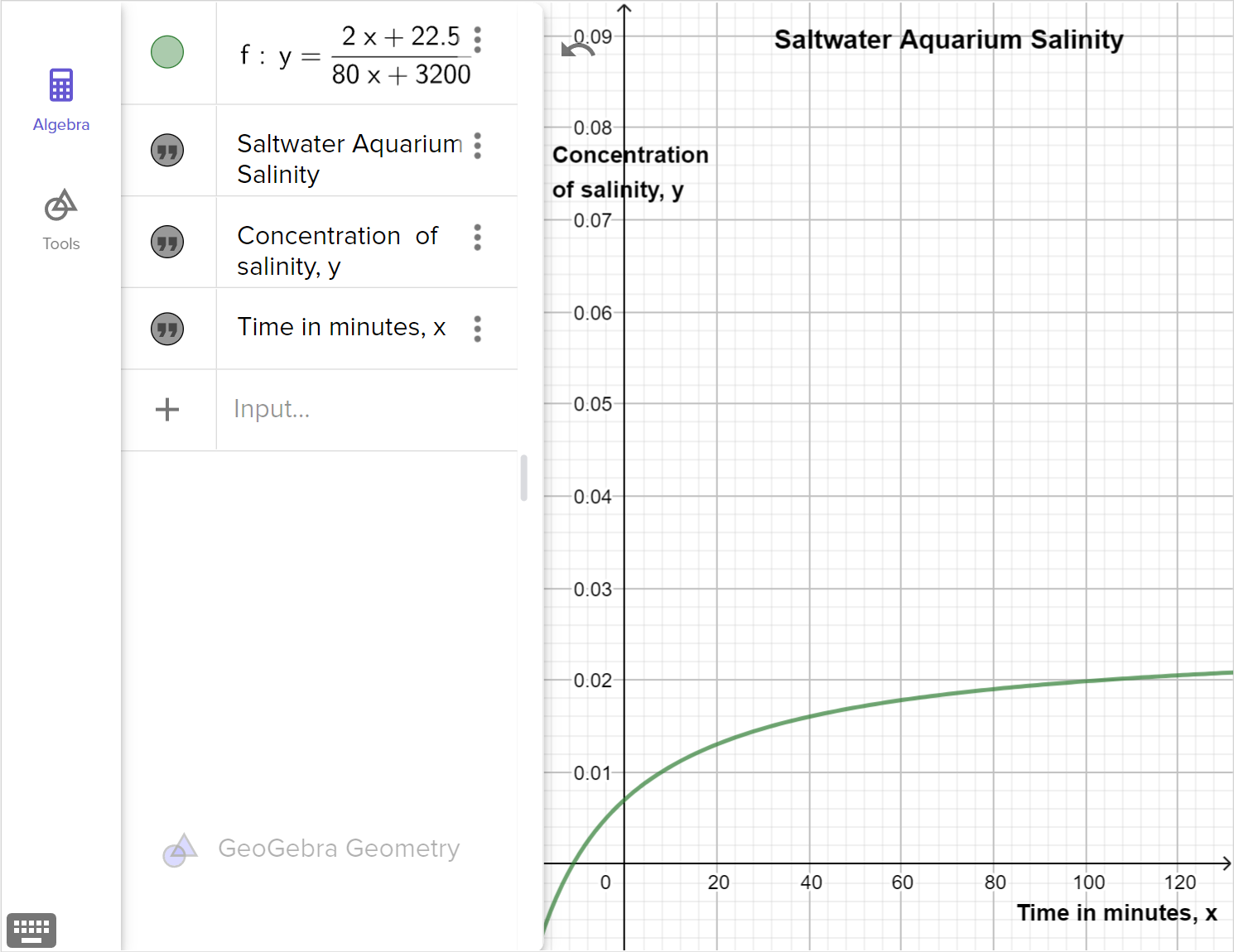
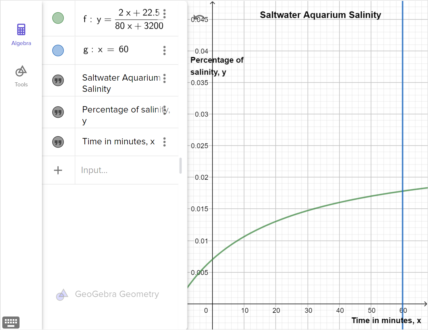
Reyita proposed the following function to model the concentration of the salt per gallon over time in the aquarium, where x represents the time in minutes and f \left(x \right) represents the cups of salt per gallon:f \left( x \right) = \dfrac{2x + 22.5}{5x+200}

The following graph models the function that shows the concentration of the saltwater:

-1600
-1400
-1200
-1000
-800
-600
-400
-200
200
400
600
800
1000
1200
1400
1600
x
0.1
0.2
0.3
0.4
0.5
0.6
0.7
0.8
0.9
f(x)

The following table models the water and salt content of the aquarium for the first 15 minutes in intervals of 5:

Time (Minutes)Water (Gallons)Salt (Cups)
020022.5
522532.5
1025042.5
1527552.5
a

Examine the equation, graph and table that model this context. Are they all accurate models of the situation? If so, explain how the model matches the context. If not, identify any problems with the model, and revise the model to address the problems.

Worked Solution
Create a strategy

It is possible to consider the representations of the context in any order. For this context, we can start by reviewing the table of values to confirm that the time, water, and salt align to the given scenario. Then, we can work with the other representations to determine their accuracy.

Apply the idea
Time (Minutes)Water (Gallons)Salt (Cups)
020022.5
522532.5
1025042.5
1527552.5

At time 0, we know that 200 \text{ gal} of water are mixed with 22.5 \text{ c} of reef salt.

A hose turned on with a rate of adding 5 \text{ gal/min} accurately shows an additional 25 \text{ gal} in the tank every 5 \text{ mins}.

Salt is poured in at a rate of 120 \text{ c/hr} but the table is in minutes, so we must convert the salt rate to cups per minute.

\dfrac{120 \text{ cups}}{1 \text{ hour}} \times \dfrac{1 \text{ hour}}{60 \text{ minutes}}= \dfrac{2 \text{ cups}}{1 \text{ minute}}

The rate at which the salt is being poured would appear in the table as 10 cups every 5 minutes, which is accurate. Finally, we should align the units of the water and salt measurements in the table so that they are more useful to us. We can change the gallons to cups by multiplying each gallon amount by \dfrac{16 \text{ cups}}{1 \text{ gallon}}.

Time (Minutes)Water (Cups)Salt (Cups)
03\,20022.5
53\,60032.5
104\,00042.5
154\,40052.5

Next, let's review Reyita's suggested function modeling the context. After reviewing the accuracy of the table of values with the given context, we can see the structure of the equation is given in the formf \left(x \right) = \dfrac{\text{total cups of salt}}{\text{total gallons of water}}= \dfrac{2x + 22.5}{5x+200}where x represents the time in minutes. This equation is accurate with those units, but using units of cups of salt per gallon of water will not help us solve the main part of the problem. We need to make sure the salinity remains between 1 \% and 3\%. In order to determine the percentage of salt in the water, the volume of the salt and the water needs to be measured with the same units.

To change from gallons of water to cups of water, we multiply the gallons by \dfrac{16 \text{ cups}}{1 \text{ gallon}}. The total gallons of water can be expressed by: 16 \left( 5x + 200 \right) = 80x + 3\,200 by the distributive property. Now we can write a function equation that represents the percentage of salt in the water:f \left(x \right) = \dfrac{\text{total cups of salt}}{\text{total cups of water}}= \dfrac{2x + 22.5}{80x+3\,200}

Finally, we'll change the function and edit the graph to use the converted units and add appropriate labels to the graph:

A screenshot of the GeoGebra tool showing the graph of y equals 2 x plus 22.5 all over 80 x plus 3,200. Speak to your teacher for more details.

For each model we should also note the domain the model is appropriate for. See part (b) for considerations of the limitations of the models.

Reflect and check

When analyzing models, we should always examine the units to make sure they make sense for the context and produce solutions that are in the desired units.

b

What are the limitations of our model in terms of the context?

Worked Solution
Create a strategy

When considering the context of the problem, we should look at aspects such as extraneous solutions or non-viable solutions. Contextual factors may also place constraints on the domain and range.

Apply the idea

The domain of the function f\left( x \right) = \dfrac{2x + 22.5}{80x+3\,200} should be restricted from any values where 80x+3\,200=0, so when x=-40. Since x is in minutes, it cannot reasonably be negative and the restriction is not relevant to the context.

The capacity of the aquarium is 500 gallons or 8\, 000 cups, so the time at which the aquarium will reach its maximum amount of water will limit the maximum value of the domain. And since time cannot be a negative value, the domain of the function starts at time 0.

8\,000 \text{ cups} - 3\,200 \text{ cups at time zero} = 4\,800 \text{ cups of water} \\ 4\,800 \text{ cups of water} \div 80 \text{ cups per minute} = 60 \text{ minutes}

The domain of the model is \left[0, 60 \right].

The range constraints should come from the domain constraints, so the range would be \left[f \left(0 \right), f \left(60 \right) \right]. We will still examine our model to make sure the salinity remains in the safe range between 1 \% and 3 \%, but it is contextually possible to have salinity rates outside of the range.

Graphing the function as a system of equations, we can visualize the domain and range restrictions in this context by examining points of intersection:\begin{cases} y = \dfrac{2x + 22.5}{80x+3\,200} \\ x=60 \end{cases}

A screenshot of the GeoGebra tool showing the graphs of y equals 2 x plus 22.5 all over 80 x plus 3,200 and x equals 60. Speak to your teacher for more details.

We could also restrict the function to the appropriate domain in Geogebra using the command: g\left(x\right)=\text{If}\left(0 \leq x \leq 60, f\left(x\right)\right) or alternatively {g\left(x\right)=\text{Function(function, start } x \text{-value, end } x \text{-value)}} with the following inputs g\left(x\right)=\text{Function}\left(f\left(x\right), 0, 60\right).

Reflect and check

The limitations of our model in terms of the context may bring up other problems that we will need to consider when interpreting results and drawing conclusions.

c

Determine the conclusions that can be drawn from our model. State assumptions that were made, if any.

Worked Solution
Create a strategy

We might assume that the mixture is safe for the fish initially, but we should check the model and confirm that it stays within an appropriate range.

We will consider the salinity of the water while it is filling and after the aquarium is full. Then, we can determine if we should make adjustments to the salt or water prior to filling the aquarium.

Apply the idea

By looking at the graph modeling the context, we can see that the salinity of the water starts below 1 \% and slowly rises into the safe range for the fish. We can also calculate the salinity of the water using our table of values and add a column:

Time (Minutes)Water (Cups)Salt (Cups)Salinity
03\,20022.50.7 \%
53\,60032.50.9 \%
104\,00042.51.1 \%
154\,40052.51.2 \%

We can see from the table and graph that the water in the tank will be safe for fish sometime just before ten minutes. So, no fish should be added to the tank before ten minutes.

We can algebraically check the salinity once the tank is full, to make sure it is still within safe bounds. f\left( 60 \right) = \dfrac{2 \left(60 \right) + 22.5}{80 \left( 60 \right) +3\,200} = \dfrac{142.5}{8\,000}= 0.0178 \approx 1.8 \%

Since the salinity of the full tank is within safe range in this case, we do not need to make any recommendations to changing the context or model.

Reflect and check

If the salinity had not been in the safe range once the aquarium was full, we could have considered adjusting the rate of pouring salt, creating different function models with different rates, and determining which model keeps the salinity between 1 \% and 3 \% when the tank is full.

Example 2

On a given day flying from New York City, NY to Los Angeles, CA, the tailwind from New York City to Los Angeles will increase the plane's speed. The return flight from Los Angeles against the wind will decrease the plane's speed. Suppose that the speed of the wind is 32 \text{ mi/hr}. The round trip flight takes anywhere from 10 hours to 12 hours and 15 minutes.

Map of the USA with two points labeled CA and NY. The distance between CA and NY is 2,450 miles.

Maelys looks up the distance to fly from NYC to LA, which is approximately 2\,450 miles. Then she creates a table, equation, and graph to model the context assuming the round trip flight is scheduled to be a total of 12 hours and 15 minutes. Maelys identifies the unknown speed of the plane in miles per hour as x, and uses this in the equation:\text{Time to LA} + \text{Time to NYC} = \text{Total Time}

A table that organizes the given data follows:

DistanceRateTime
Tailwind2\,450 \text{ miles}x + 32 \text{ mi/hr}\dfrac{2\,450}{x+32}
Headwind2\,450 \text{ miles}x- 32 \text{ mi/hr}\dfrac{2\,450}{x-32}

The equation that Maelys writes to model the context and can be used to find the speed of the plane is: \dfrac{2\,450}{x+32} + \dfrac{2\,450}{x-32} = 12.25

Finally, Maelys uses technology to graph the function for the speed of the plane when the trip takes 12 hours and 15 minutes:

Round trip flight from NYC to LA
-300
-250
-200
-150
-100
-50
50
100
150
200
250
300
350
400
450
\text{Speed in miles per hour, }x
-150
-100
-50
50
100
150
200
250
300
350
\text{Total time, }T\left(x\right)
a

Examine the equation, graph and table that model this context. Are they all accurate models of the situation? If so, explain how the model matches the context. If not, identify any problems with the model, and revise the model to address the problems.

Worked Solution
Create a strategy

The table created by Maelys is used to construct the equation, so we want to make sure the units of the table are aligned and make sense in context. Then, we should follow up with the units of the equation and determine the accuracy of the graph.

Apply the idea

Maelys sets up a table of values for distance, rate, and time in order to use the formula \text{Distance}= \text{Rate} \times \text{Time}. We can assume that if she researched the total distance, that the flight will be nonstop between destinations and that the route is the same there and back. The tailwind will add speed to the flight and the headwind will reduce the speed, so the rate column is accurate.

The formula can be rewritten as \text{Time}=\dfrac{\text{Distance}}{\text{Rate}}, so the entries in the final column of the table are written as \dfrac{\text{Distance}}{\text{Rate}}.

Maelys appropriately writes a math sentence with words to show the equation that she is using to model the speed of the plane, so we can add the time in one direction to the time to fly in the opposite direction for a total of 12 hours and 15 minutes, or 12.25 hours.

The units for the equation also make sense, as it is written as \dfrac{\text{miles}}{\text{miles per hour}}+\dfrac{\text{miles}}{\text{miles per hour}} = \text{hours}

Finally, Maelys rewrites the equation as T \left(x \right)= \dfrac{2\,450}{x+32} + \dfrac{2\,450}{x-32} - 12.25 and the graph has appropriate labels on the axes and for its title.

Subtracting the 12.25 creates a function where the x-intercepts of the graph will help us find the speed of the plane for a 12.25-hour round trip.

b

Determine the average speed of the plane if the total trip time is 12 hours and 15 minutes, and interpret the results.

Worked Solution
Create a strategy

As we discussed in the previous part, the function model T \left(x \right)= \dfrac{2\,450}{x+32} + \dfrac{2\,450}{x-32} - 12.25 can be used to find the speed of the plane for a 12.25-hour trip.

We must exclude x=-32 and x=32 from the domain. Since x=-32 is negative, it is not relevant to the problem since negative speeds would not make sense. However, since x=32 will lead to an undefined solution, we must exclude it from the solution as it is an asymptote.

Apply the idea

Let's find the x-intercepts of the function in Maelys' graph to determine the speed of the plane. We can write the equation as \dfrac{2\,450}{x+32} + \dfrac{2\,450}{x-32} - 12.25 = 0 and solve for x.

\displaystyle \dfrac{2\,450}{x+32} + \dfrac{2\,450}{x-32} - 12.25\displaystyle =\displaystyle 0Equation for the speed of the plane for a 12 hours and 15 minute round trip
\displaystyle \dfrac{x -32}{x-32} \cdot \dfrac{2\,450}{x+32} + \dfrac{x +32}{x+32} \cdot\dfrac{2\,450}{x-32} + \dfrac{\left(x+32 \right) \left(x -32 \right)}{\left(x+32 \right) \left(x -32 \right)} \cdot -12.25\displaystyle =\displaystyle 0Calculate a common denominator
\displaystyle \dfrac{2\,450x - 78\,400}{\left(x+32 \right) \left(x -32 \right)} + \dfrac{2\,450x + 78\,400}{\left(x+32 \right) \left(x -32 \right)} + \dfrac{-12.25x^2 + 12\,544}{\left(x+32 \right) \left(x -32 \right)}\displaystyle =\displaystyle 0Multiply the rational expressions
\displaystyle \dfrac{12.25x^2 + 4\,900x - 12\,544}{\left(x+32 \right) \left(x -32 \right)}\displaystyle =\displaystyle 0Add the rational expressions
\displaystyle 12.25x^2 + 4\,900x - 12\,544\displaystyle =\displaystyle 0Multiply both sides by \left(x+32 \right) \left(x -32 \right)

We can use the quadratic formula to find the value of x:

\displaystyle x\displaystyle =\displaystyle \frac{-b\pm \sqrt{b^2-4ac}}{2a}State the quadratic formula
\displaystyle =\displaystyle \frac{-\left(4\,900\right)\pm \sqrt{\left(4\,900\right)^2-4\left(-12.25\right)\left(12\,544\right)}}{2\left( -12.25\right)}Substitute a=-12.25, b=4\,900, c=12\,544
\displaystyle =\displaystyle \frac{-4\,900\pm \sqrt{24\,624\,656}}{-24.50}Evaluate the square, products and the difference
\displaystyle =\displaystyle -2.5 \text{ and } 402.5 \text{ mi/hr}Evaluate the sum and quotient, and then evaluate the difference and quotient

-2.5 miles per hour is an extraneous solution because the plane cannot have a negative speed. So, this intercept is non-viable in context. For the plane to make a 12.25-hour round trip, it will fly at an average speed of 402.5 \text{ mi/hr}.

c

Revise the model to be useful for comparing any trip times within the given range. Describe any limitations or assumptions in the model.

Worked Solution
Create a strategy

We need to consider potential contextual and mathematical limitations on the domain and range.

In this context, it does not make sense to talk about negative speeds or negative time. We also do not need to consider speeds that will cause the plane to fly more than 12 hours and 15 minutes, which will be the highest end limit of our range.

If we examine the graph between 0 and 32 \text{ mi/hr}, which is an excluded value of our domain due to its asymptote, we can see that the time, T \left( x \right), has negative values, which does not make sense in our context. We need to examine what is happening at lower speeds of the plane.

An internet search shows that a commercial plane does not take off from the ground until it reaches between 160 and 180 \text{ mi/hr}. So, speeds below 160 \text{ mi/hr} should not be considered part of our domain.

Apply the idea

We need a model that will look at speeds for trip lengths between 10 hours and 12.25 hours. We could change her function model to a system of equations.\begin{cases} y = \dfrac{2\,450}{x+32} + \dfrac{2\,450}{x-32} \\y=12.25 \\ y=10 \end{cases}

The graphical model that Maelys uses also limits the length of the trip. We could change Maelys' graph and graph the system of equations instead, so that we can determine the speed of the plane given different time estimates, as follows:

A screenshot of the GeoGebra tool showing the graphs of y equals 2,450 over x plus 32 plus 2,450 over x minus 32 minus 12.3, y equals 12.25, and y equals 10. Speak to your teacher for more details.

By adjusting Maelys' model, this system of equations and graph would model any specified trip times. We already know the slowest speed will be 402.5 \text{ mi/hr} for a 12.25-hour trip. For a 10-hour hour trip, using the graph to find the intersection point, we get a speed of 492.1 \text{ mi/hr}. Therefore, the domain is \left[402.5, 492.1 \right] with a corresponding range of \left[10, 12.25 \right].

This model will give us approximate values to the actual speeds and times, since it doesn't account for take-off and landing times or time on the ground, and assumes a constant distance of 2\,450 miles in each direction, and a constant wind speed in both directions.

Reflect and check

This is not a complete solution for the limitations on the model, but examples that can be taken into consideration when attempting to model a real world context with mathematics.

Idea summary

The ability to interpret the results of a model and make evidence-based decisions is an important part of the modeling process. We can always utilize new information, or re-examine existing information, to make improvements to a model, influencing further decisions.

Outcomes

AII.7g

Investigate and analyze linear, quadratic, absolute value, square root, cube root, rational, polynomial, exponential, and logarithmic function families algebraically and graphically for the concept of connections between and among multiple representations of functions using verbal descriptions, tables, equations, and graphs

What is Mathspace

About Mathspace