7. Two Variable Statistics

7.02 Fitting functions to data

Lesson

Practice

7.03 Analyzing fitted functions

Book a Demo

United States of America

Grades 9-12

7.02 Fitting functions to data

Lesson

Practice

Introduction

We sketched and interpreted lines of best fit in lesson 7.01 Scatter plots and lines of fit . We will learn how to calculate the line of best fit and the correlation coefficient using technology and then extend the concept to modeling exponential relationships.

Ideas

Fitting functions to data

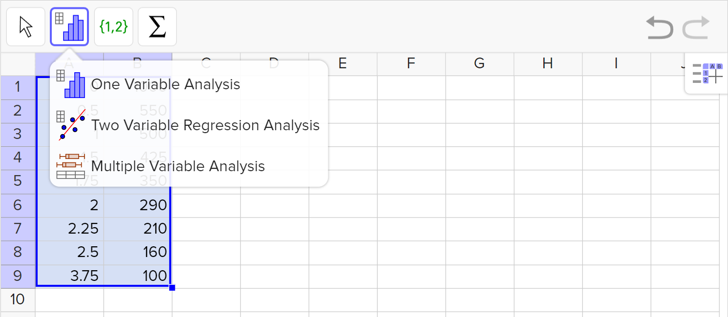
Fitting functions to data

Exploration

Use the linear and exponential models to fit the data on the graph.

Loading interactive...

Which function fits the data better? How do you know?

Sometimes we need to consider fitting something other than a line of best fit or regression line, which both refer to a linear regression model, to model data. A fitted function could include another type of function, such as an exponential function.

We already learned about the correlation coefficient, r, a statistic that describes both the strength and direction of a linear association. But, we also need a measure that determines how well our fitted function can actually predict an outcome.

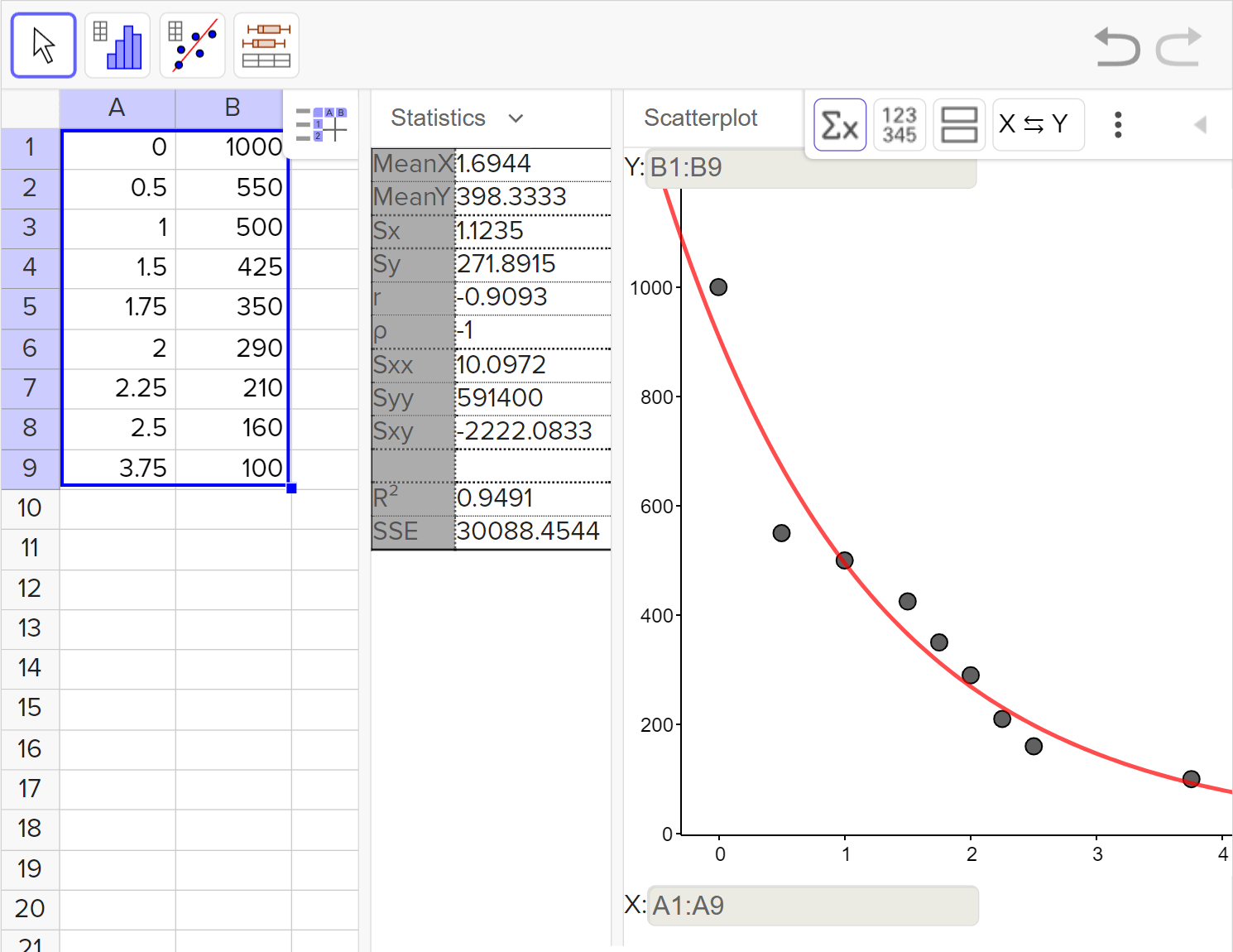
This value is known as the coefficient of determination, or the value R^2, and is a measure of the proportion of the variation in the dependent variable that is predicted by the independent variable. Since the coefficient of determination represents a proportion it will only ever return a value between 0 and 1.

In the case where the fitted function is a linear model with one independent variable, R^2 is equal to our correlation coefficient squared, r^2. This only holds true for linear models with one independent variable and is not the case when the fitted function is from any other function family, e.g. exponential, quadratic, etc.

Coefficient of determination

A measurement used to explain how much the variability of one quantity can be explained by its relationship to another quantity

Bivariate data can be modeled with a fitted function also called a regression model. Depending on the goodness of fit, measured with the coefficient of determination (R^2), a regression function may pass exactly through all of the points, some of the points, or none of the points.

0.1

0.2

0.3

0.4

0.5

10000

20000

30000

40000

50000

\text{ Exponential regression } R^2=0.763

R^2 for the exponential regression shown means that 76.3\% of the variation in the dependent variable is explained by the variation in the independent variable. The closer R^2 is to 1, the more that the variation in the dependent variable is explained by the variation in the independent variable.

Examples

Example 1

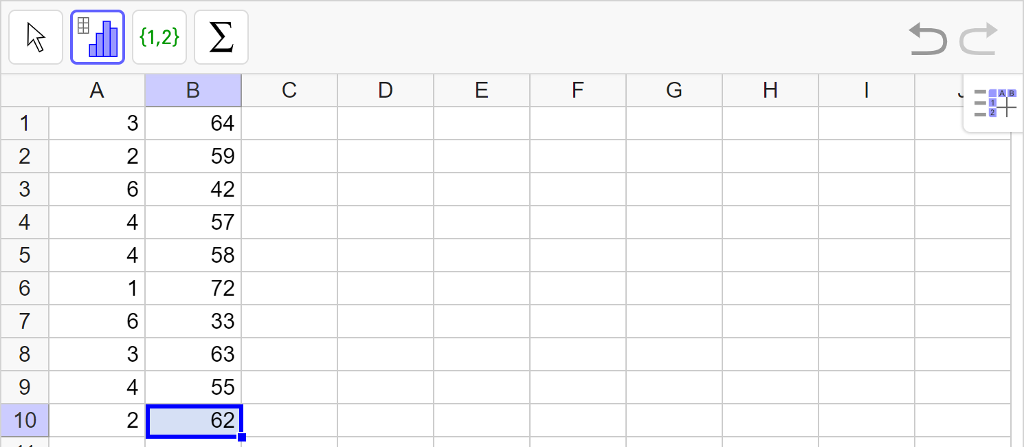
A teacher recorded the number of days since a student last studied for an exam and their score out of a possible 80 points on the exam.

Number days since studying	3	2	6	4	4	1	6	3	4	2
Exam score	64	59	42	57	58	72	33	63	55	62

Describe the association between the number of days since student and the exam score.

Worked Solution

Create a strategy

Construct a scatterplot to get a visual of the data.

\text{Days since studying}

\text{Score }

Then consider the form, strength, and direction.

Apply the idea

The data appears to have a strong, negative, linear association.

Calculate the line of best fit and correlation coefficient. Interpret the correlation coefficient.

Worked Solution

Create a strategy

Enter the x- and y-values in two separate columns:
Highlight the data and select Two Variable Regression Analysis:
Select Show Statistics to see the correlation coefficient, r:
Choose Linear under the Regression Model drop down menu to find the line of best fit:

Apply the idea

The equation of the line of best fit is y=-6.22x+78

The correlation coefficient is r=-0.9115, meaning that there is a strong negative correlation between the number of days since a student last studied and their score on the exam.

Reflect and check

The correlation coefficient provides statistical evidence for the association.

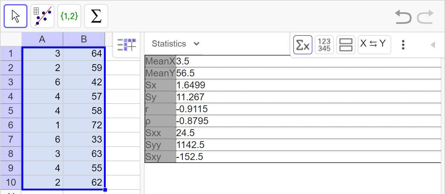
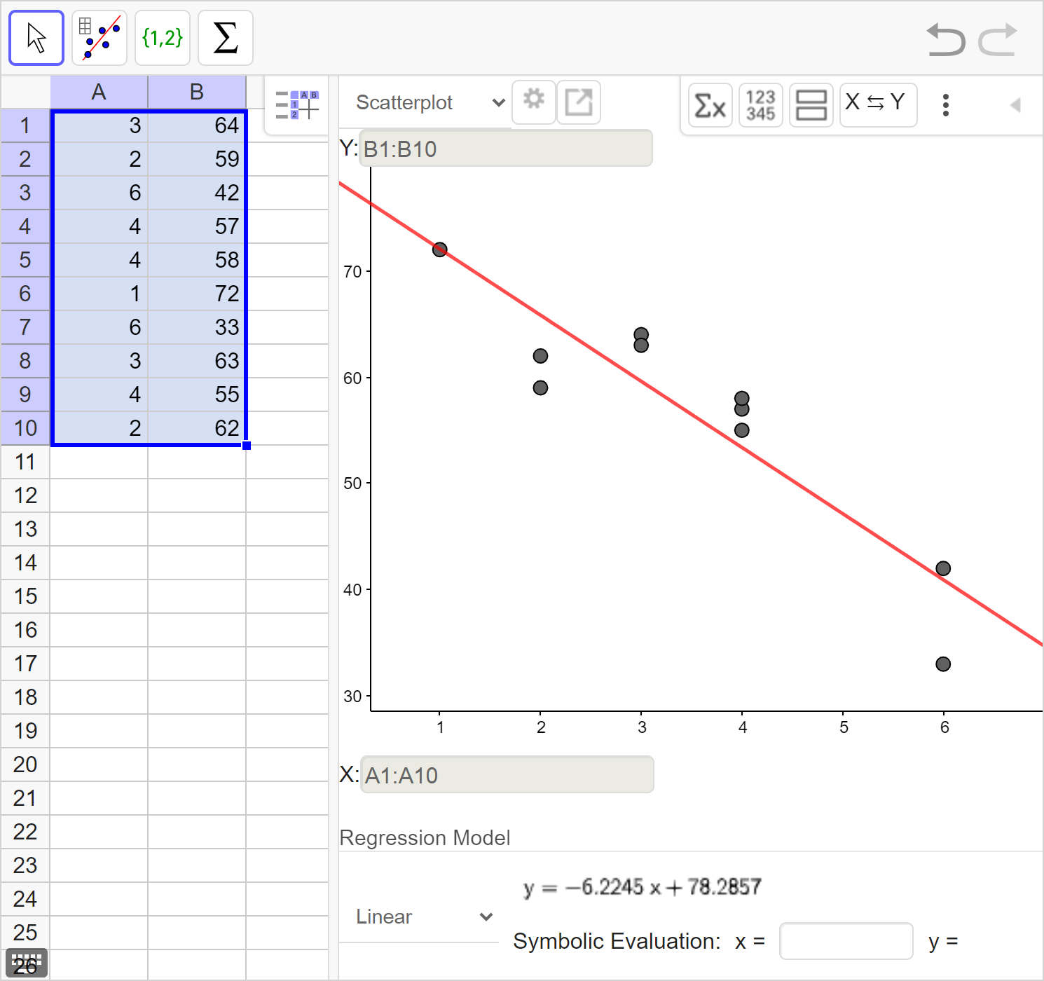
Interpret the meaning of the slope and y-intercept of the line of best fit in context of the data.

Worked Solution

Create a strategy

From part (b) we know that the equation of the line of best fit is y=-6.22x+78 which tells us the slope is -6.22 and the y-intercept is 78.

Apply the idea

The slope of -6.22 represents the driving score dropping by -6.22 points each day gone without studying.

The y-intercept tells us that a studen who has studied with 0 days to the exam has a predicted score of 78 according to the linear model.

Reflect and check

Matching the slope and the y-intercept to their respective units is a good strategy for interpreting their meaning in context. \text{slope}=\dfrac{\text{rise}}{\text{run}}=\dfrac{-6.22}{1}

The quantity on the y-axis represents the "rise" and the quantity on the x-axis represents the "run". So the slope represents negative 6.22 score for every 1 day.

The y-intercept can be written as an ordered pair \left(x,y\right)=\left(0,78\right) where x is the number of days since studying and y is the exam score.

Example 2

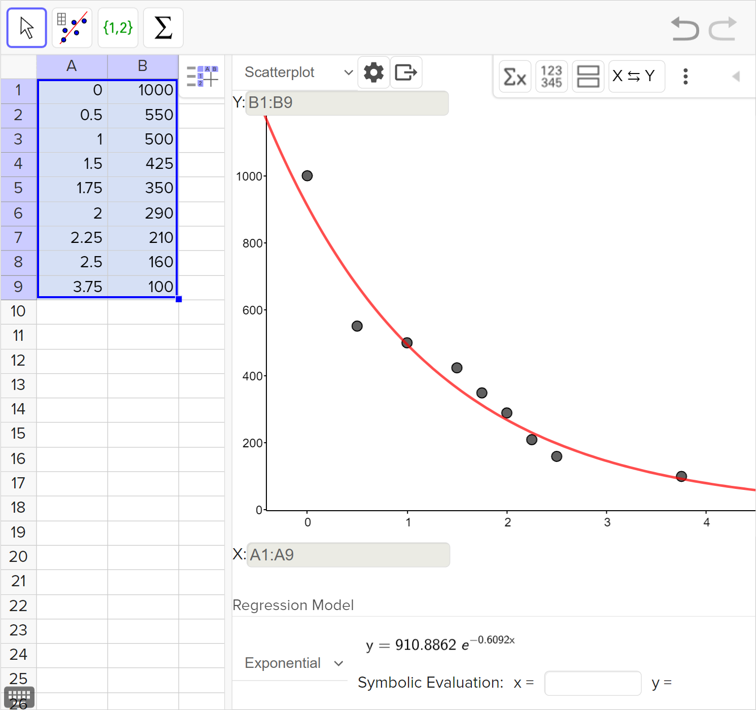
The population P of fish in a small lake over t years is shown in the table below:

Years (t)	Fish Population (P)
0	1000
0.5	550
1	500
1.5	425
1.75	350
2	290
2.25	210
2.5	160
3.75	100

Determine whether a linear or exponential model best fits the relationship between the years, t, and the population of fish P.

Worked Solution

Create a strategy

Plot the data on a coordinate plane and examine the shape of the data.

Lake Fish Population

\text{Years }t

100

200

300

400

500

600

700

800

900

1000

\text{Population }P

Apply the idea

An exponential model would best fit the data after examining the plot.

Calculate the regression model for the data and use it to predict the population of fish in the lake after 5 years.

Worked Solution

Create a strategy

Use technology to calculate the exponential regression, then use the equation to determine the population when t=5.

Enter the x- and y-values in two separate columns, then highlight the data and select Two Variable Regression Analysis :
Choose Exponential under the Regression Model drop down menu to find the line of best fit:

Apply the idea

The function that fits the model best is P=910.9e^{-0.61t}

If t=5, then P=910.9e^{-0.61 \cdot 5}=43.14. This means that according to the regression model, we can expect there to be about 43 fish remaining in the lake after 5 years.

Interpret the coefficient of determination for the regression model.

Worked Solution

Create a strategy

From the calculated regression model in the calculator, select Show Statistics to see the coefficient of determination, R^2:

A screenshot of the GeoGebra statistics tool showing the following: On the left side: the numbers 0, 0.5, 1, 1.5, 1.75, 2, 2.25, 2.5, and 3.75 in column A, rows 1 to 9 and the numbers 1000, 550, 500, 425, 350, 290, 210, 160, and 100 in column B, rows 1 to 9. On the middle: a list of statistical values is shown. On the right side: a scatterplot and the best fit curve are shown. Speak to your teacher for more details.

Apply the idea

The coefficient of determination is 0.9491, meaning that 94.91 \% of the variation in the fish population is explained by the variation in the year that the measurement was taken.

Reflect and check

In our statistics table we can see we produced a value for the correlation coefficient r and the coefficient of determination R^2.

From our statistics table we can see that if we take the square of r, we get r^2 is equal to 0.8268. However, in the statistics table R^2 equals 0.9491. These values are not equal since our fitted function is an exponential function and not a linear function.

If we instead selected Linear under the Regression Model drop down, we would obtain the same value for the correlation coefficient since it is a measure of linear association regardless of the function type we choose, however our value for R^2 would instead have been 0.8268. Notice that this value is equal to r^2 in the linear case.

Idea summary

Linear and exponential data can be fitted to a regression model. We can analyze the closeness of the fit using the coefficient of determination.

Outcomes

S.ID.B.6.A

Fit a function to the data; use functions fitted to data to solve problems in the context of the data. Use given functions or choose a function suggested by the context. Emphasize linear, quadratic, and exponential models.

S.ID.C.7

Interpret the slope (rate of change) and the intercept (constant term) of a linear model in the context of the data.

S.ID.C.8

Compute (using technology) and interpret the correlation coefficient of a linear fit.

7.02 Fitting functions to data

Introduction

Ideas

Fitting functions to data

Exploration

Examples

Example 1

Example 2

Outcomes

S.ID.B.6.A

S.ID.C.7

S.ID.C.8

What is Mathspace

About Mathspace