topic badge

8.01 Comparing functions across representations

Introduction

We have learned about key features of functions in Algebra 1 and throughout Algebra 2. These key features also apply to functions that represent real-world contexts. This lesson aims to compare functions represented in different ways and determine which functions best model real-world phenomena.

Comparing functions across representations

Functions can be represented in a variety of ways, including equations, tables, and graphs. It is important to be able to compare functions whether they are represented in similar or different ways.

Useful information can usually be obtained by comparing key features of the functions. Remember that key features include:

  • Domain and range

  • Intercepts

  • End behavior

  • Rate of change

  • Maximum or minimum value(s)

  • Positive and negative intervals

  • Increasing and decreasing intervals

  • Asymptote(s)

  • Axis of symmetry

Recall the function families we have studied throughout Algebra 2:

Functions with their general equations and graphs shown below. From left to right, the functions are: Linear, f of x equals x; Quadratic, f of x equals x squared; Square root, f of x equals square root of x; Cubic, f of x equals x cubed; and Cube root, f of x equals cube root of x. Speak to your teacher for more details.
Functions with their general equations and graphs shown below. From left to right, the functions are: Absolute value, f of x equals absolute value of x; Rational-Linear, f of x equals 1 over x; Rational-Quadratic, f of x equals 1 over x squared; Exponential, f of x equals b raised to x where b is greater than 1; and Logarithmic, f of x equals log of x base b when b greater than 1. Speak to your teacher for more details.

Examples

Example 1

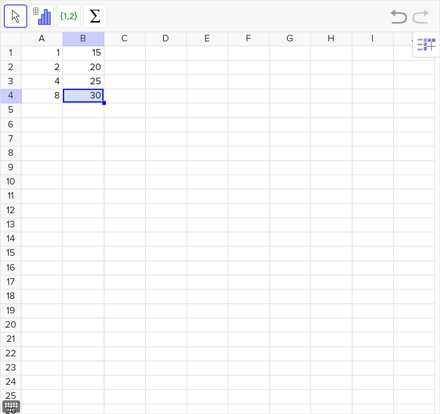
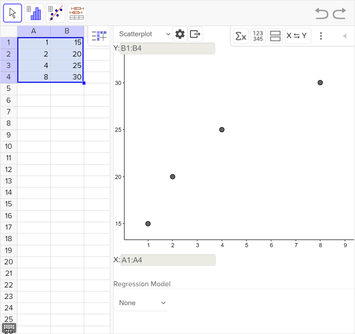
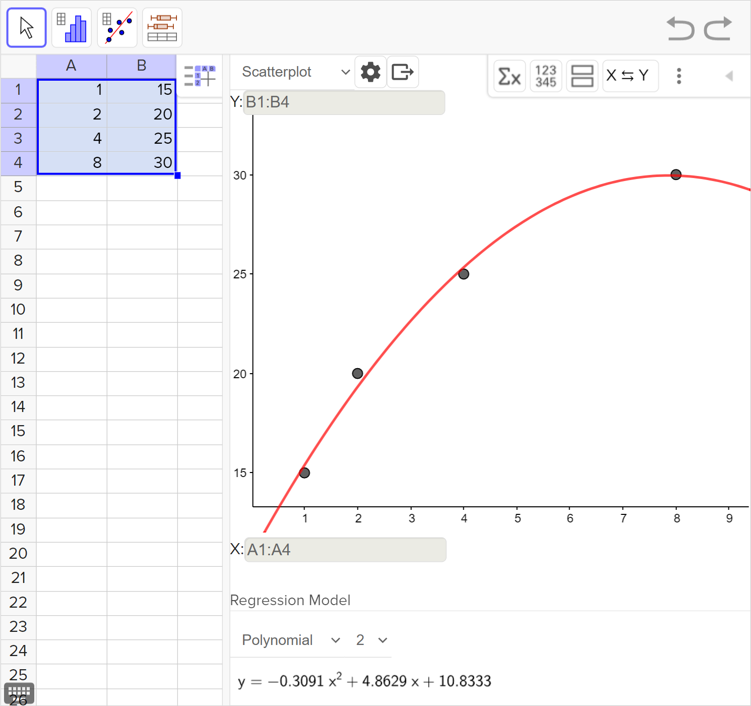
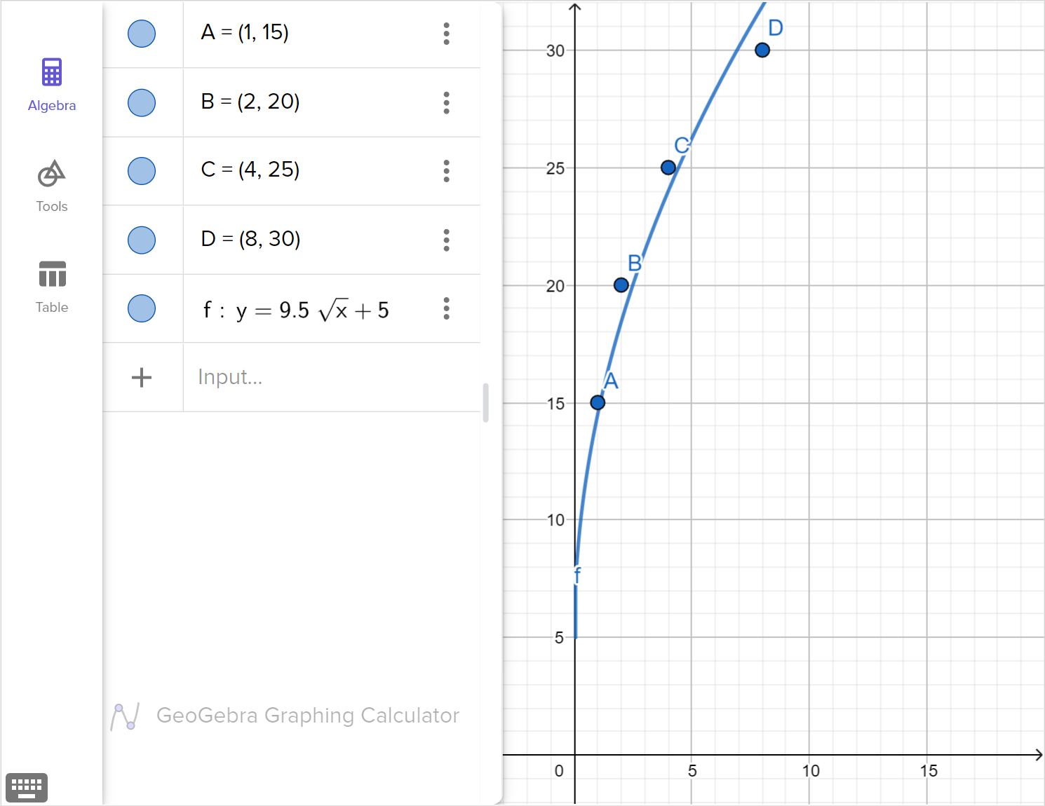
Nasrin decides to start doing home exercises and records the number of push-ups that they can do in one attempt at the end of a given week. Their results are shown in the table.

Week1248
Push-ups15202530
a

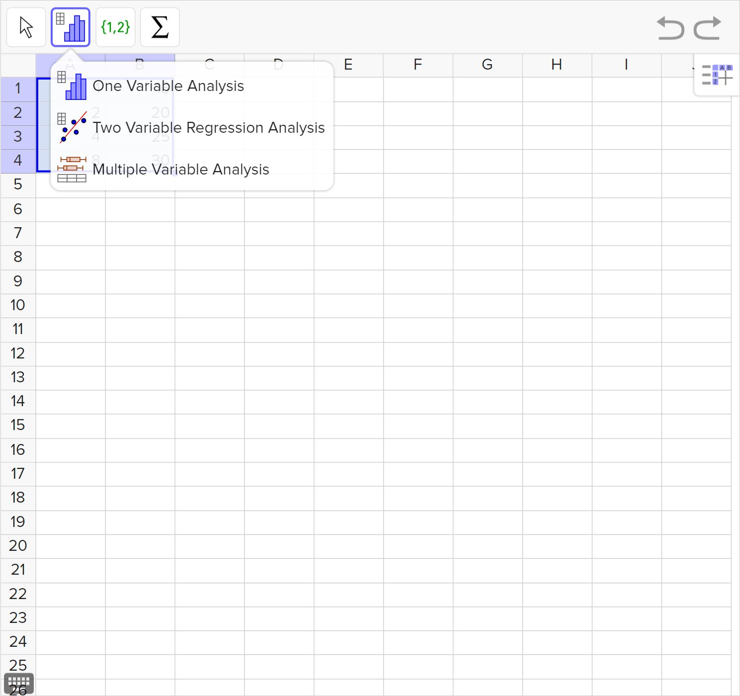
Choose which of the following functions would model Nasrin's exercise chart best: a radical function, a rational function, quadratic function, or a logarithmic function.

Worked Solution
Create a strategy

Graph the data on a coordinate plane and determine which regression model fits best.

In order to find the regression curve, we can input the x and y values into a table, then use the Two-Variable Statistics tool and choose a model:

A screenshot of the GeoGebra statistics tool showing the data 1, 2, 4, and 8 entered in column A, rows 1 to 4, and 15, 20, 25, and 30 entered in column B, rows 1 to 4. Speak to your teacher for more details.
A screenshot of the GeoGebra statistics tool showing the data 1, 2, 4, and 8 entered in column A, rows 1 to 4, and 15, 20, 25, and 30 entered in column B, rows 1 to 4. The cells from column A, rows 1 to 4, and column B, rows 1 to 4, are selected. The menu from the second leftmost icon is shown.
A screenshot of the GeoGebra statistics tool showing the following: On the left side: the numbers 1, 2, 4, and 8 entered in column A, rows 1 to 4, and 15, 20, 25, and 30 entered in column B, rows 1 to 4. The cells from column A, rows 1 to 4, and column B, rows 1 to 4, are selected. On the right side: a scatterplot is shown. Speak to your teacher for more details.
Apply the idea
Nasrin's push-up record
1
2
3
4
5
6
7
8
\text{Weeks, }x
5
10
15
20
25
30
35
\text{Push-ups, }y

The shape of the graph could lend itself to any of the given functions, since the graph shows that the number of push-ups Nasrin can do increases at a decreasing rate.

We can take key features into consideration when choosing a model. We might note that the domain and range of a square root function are always positive, so a radical function could fit our data. We could, however, restrict the domain and range of any of the functions.

The regression model for a logarithmic function follows:

A screenshot of the GeoGebra statistics tool showing the following: On the left side: the numbers 1, 2, 4, and 8 entered in column A, rows 1 to 4, and 15, 20, 25, and 30 entered in column B, rows 1 to 4. The cells from column A, rows 1 to 4, and column B, rows 1 to 4, are selected. On the right side: a scatterplot and the best fit curve are shown. Speak to your teacher for more details.

The regression model for a quadratic function follows:

A screenshot of the GeoGebra statistics tool showing the following: On the left side: the numbers 1, 2, 4, and 8 entered in column A, rows 1 to 4, and 15, 20, 25, and 30 entered in column B, rows 1 to 4. The cells from column A, rows 1 to 4, and column B, rows 1 to 4, are selected. On the right side: a scatterplot and the best fit curve are shown. Speak to your teacher for more details.

Another option for fitting models is adding the points to a graph and building a transformed parent function using our knowledge of transformations of functions. This is not as accurate as using a regression model, but the functions can be manipulated to follow the shape of our data.

A potential radical function follows:

A screenshot of the GeoGebra graphing calculator showing the points A at (1,15), B at (2, 20), C at (4, 25), D at (8,30), and the graph of y equals 9.5 square root of x plus 5. Speak to your teacher for more details.

A potential rational function follows:

A screenshot of the GeoGebra graphing calculator showing the points A at (1,15), B at (2, 20), C at (4, 25), D at (8,30), and the graph of y equals negative 50 over x plus 1.5 plus 35. Speak to your teacher for more details.

Given the various function models, the logarithmic function fits Nasrin's charted exercise data the best.

b

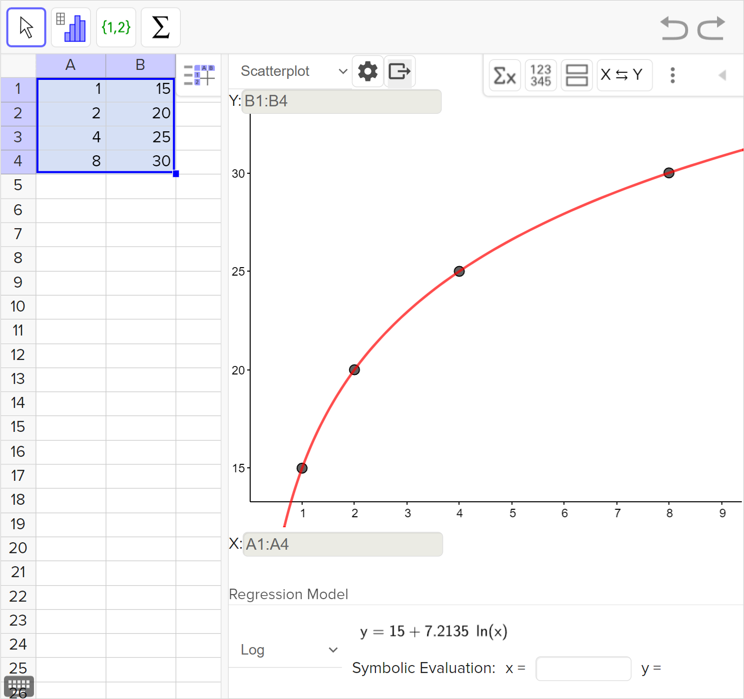
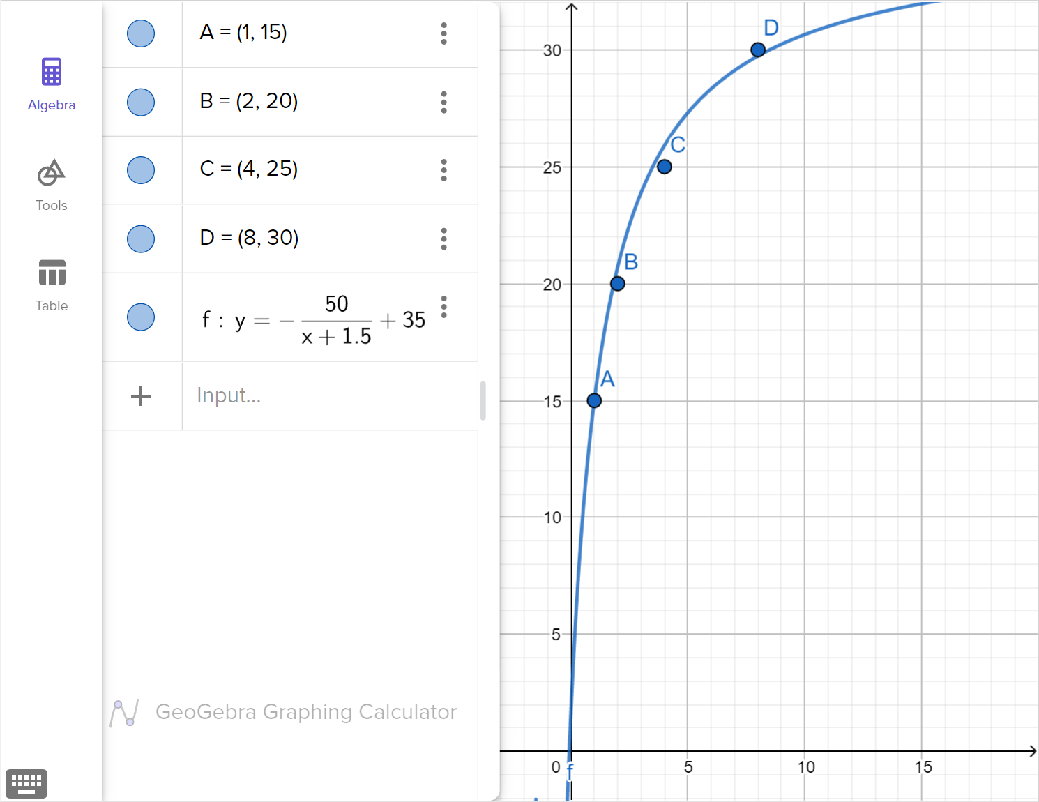
State the number of push ups that Nasrin will be able to do after 16 weeks, according to the model you chose in part (a).

Worked Solution
Create a strategy

Use the equation given for the regression curve of a logarithmic function and substitute 16 for x.

Apply the idea

The equation that best models Nasrin's push-up routine is given by y=15 + 7.2135 \ln \left( x \right). By substituting x=16, we get y=35, meaning that Nasrin will be able to do 35 push-ups in 16 weeks.

Reflect and check

We could also follow the pattern in the given data set, which shows the weeks doubling and the push-ups increasing by 5. By continuing the pattern in the set of data, we can also conclude that Nasrin will be able to do 35 push-ups in 16 weeks. By using the equation that models the context, we are verifying that the equation is a good fit.

Week124816
Push-ups1520253035

Example 2

The graph of function f \left(x \right) shown below follows the vertical height of Ameth's golf ball after being hit into the air and falling on the fairway:

Ameth's golf ball
1
2
3
4
\text{Time (seconds), } x
2
4
6
8
10
12
\text{Height (feet), } f \left(x \right)

The equation of function g \left(x \right) shown below follows the vertical height of Massiel's golf ball after being hit into the air and rolling through a sand trap, then out onto the green:g(x) = \begin{cases} 14 \sin \frac{3}{4}x, & 0 < x < 4 \\ \frac{1}{2} \left(x-6 \right) ^2, & 4 \leq x < 7.5 \\ -\frac{1}{4}x +3, & 7.5 \leq x < 12 \end{cases}

a

Determine whose ball is falling at a faster rate from 2 to 3 seconds.

Worked Solution
Create a strategy

Calculate the average rate of change for both functions over the interval \left[2, 3 \right], then compare.

Apply the idea

For f \left(x \right), we know that f \left( 2 \right) = 12 and f \left(3 \right)=9, so we have \dfrac{ f\left(3 \right) - f \left( 2 \right)}{3-2} = \dfrac{9 - 12 \text{ feet}}{3-2 \text{ seconds}} = \dfrac{-3 \text{ feet}}{1\text{ second}}

For g \left( x \right) over the interval \left[2, 3 \right], we must use 14 \sin \frac{3}{4}x. So g \left( 2 \right) = 13.96 and g \left( 3 \right) = 10.89, so we have \dfrac{ g\left(3 \right) - g \left( 2 \right)}{3-2} = \dfrac{10.89 - 13.96 \text{ feet}}{3-2 \text{ seconds}} = \dfrac{-3.07 \text{ feet}}{1\text{ second}}

Based on the average rate of change, Massiel's ball is falling faster 2–3 seconds after it has been hit.

b

Determine which part of the function g \left(x \right) shows the ball's vertical height in the sand trap.

Worked Solution
Create a strategy

Graph g \left( x \right), then interpret the piecewise function graphically.

Apply the idea
Massiel's golf ball
1
2
3
4
5
6
7
8
9
10
11
12
13
\text{Time (seconds), } x
2
4
6
8
10
12
14
\text{Height (feet), } f \left(x \right)

After seeing the vertical height of the ball graphically, we can break the three parts of Massiel's ball trajectory into the three functions of the piecewise function. Initially, Massiel's ball follows a path similar to Ameth's as it is hit into the air. Then, it rolls into a sand trap and back out onto the green.

The part of g \left( x \right) that shows the ball's height in the sand trap is \frac{1}{2} \left( x-6 \right) ^2.

Reflect and check

Different representations of a given function may help us to interpret contextual situations better.

c

Determine whose ball goes higher.

Worked Solution
Create a strategy

Compare the maximum values of graphs of Ameth's ball and Massiel's ball.

Apply the idea

Ameth's ball reaches a maximum height of 12 \text{ ft} while Massiel's ball reaches a maximum height of 14 \text{ ft}. Massiel's ball goes higher.

Idea summary

Real-world contexts can be modeled by various types of functions. We can compare different types of models for contextual situations using their key features:

  • Domain and range

  • Intercepts

  • End behavior

  • Rate of change

  • Maximum or minimum value(s)

  • Positive and negative intervals

  • Increasing and decreasing intervals

  • Asymptote(s)

  • Axis of symmetry

Outcomes

F.IF.B.4

For a function that models a relationship between two quantities, interpret key features of graphs and tables in terms of the quantities, and sketch graphs showing key features given a verbal description of the relationship. Key features include: intercepts; intervals where the function is increasing, decreasing, positive, or negative; relative maximums and minimums; symmetries; end behavior; and periodicity.

F.IF.B.5

Relate the domain of a function to its graph and, where applicable, to the quantitative relationship it describes.

F.IF.B.6

Calculate and interpret the average rate of change of a function (presented symbolically or as a table) over a specified interval. Estimate the rate of change from a graph.

F.IF.C.9

Compare properties of two functions each represented in a different way (algebraically, graphically, numerically in tables, or by verbal descriptions).

What is Mathspace

About Mathspace