topic badge

5.01 Exponential functions

Introduction

A linear function can be used to describe relations that increase or decrease by a constant amount over time. However, many relations increase or decrease by different amounts over time. We will investigate one of those types of functions, called exponential functions, and explore the unique way in which the outputs change over time.

Characteristics of exponential functions

Exponential relationships include any relations where the outputs increase by a constant factor or decrease by a constant factor for consistent changes in x.

An exponential relationship can be modeled by a function with the independent variable in the exponent, known as an exponential function:

\displaystyle f\left(x\right)=ab^x
\bm{a}
Leading coefficient
\bm{b}
Base where b>0, b\neq 1
\bm{x}
Independent variable
\bm{f(x)}
Dependent variable

Exploration

Consider the following equations with a=1:

y=\left(5\right)^x

x-2-1012
y\dfrac{1}{25}\dfrac{1}{5}1525

y=\left(\dfrac{1}{5}\right)^x

x-2-1012
y2551\dfrac{1}{5}\dfrac{1}{25}

y=\left(-5\right)^x

x-2-1012
y\dfrac{1}{25}-\dfrac{1}{5}1-525

y=\left(1\right)^x

x-2-1012
y11111

For each of the functions, think about the following questions:

  1. What happens to y as x increases?
  2. What is the y-intercept for each of the functions?
  3. Does the function have an x-intercept?

We can determine whether a function is exponential by dividing consecutive function values to see if they have a constant factor.

The base, or constant factor, is the number being multiplied repeatedly. It tells us how quickly the output values are growing or shrinking. We can find the base by dividing a term by the previous term, as shown below:

A table with 2 rows titled x and f of x, and with 4 columns. The data is as follows: First row: 0, 1, 2, and 3; Second row: 1, 3, 9, and 27. Below the second row are 3 semi circle arrows, each labeled times 3: from the cell containing 1 to the cell containing 3, from 3 to 9, and from 9 to 27. Below each semi circle arrows is a row of equations titled constant factor: below the left semi circle arrow, 3 divided 1 equals 3; below the middle semi circle arrow, 9 divided by 3 equals 3; below the right semi circle arrow, 27 divided by 3 equals 3.

In this example, we see that the function is growing exponentially. A function grows exponentially when it increases by a constant factor.

Exponential functions change at a faster rate than linear functions. In the table below, we are adding 3 to each term, but the terms do not grow as quickly.

A table with 2 rows titled x and f of x, and with 4 columns. The data is as follows: First row: 0, 1, 2, and 3; Second row: 1, 4, 7, and 10. Below the second row are 3 semi circle arrows, each labeled plus 3: from the cell containing 1 to the cell containing 4, from 4 to 7, and from 7 to 10.

All exponential functions of the form y=ab^x have the following features in common:

  • The domain is -\infty <x<\infty.
  • The y-intercept is at (0,a).
  • There is a horizontal aysmptote at y=0.
Asymptote

A line that a curve or graph approaches as it heads toward positive or negative infinity.

x
y

An exponential function can get infinitely close to an asymptote, but it can never cross it. This means that an exponential function of this form will not have an x-intercept.

Examples

Example 1

Consider the table of values for the function y = 2\left(\dfrac{1}{3}\right)^{ x }.

x-5-4-3-2-101234510
y486162541862\dfrac{2}{3}\dfrac{2}{9}\dfrac{2}{27}\dfrac{2}{81}\dfrac{2}{243}\dfrac{2}{59\,049}
a

Describe the behavior of the function as x increases.

Worked Solution
Create a strategy

We want to identify if the values of y are increasing or decreasing as x increases.

Apply the idea

As x increases, the function decreases at a slower and slower rate.

Reflect and check

We can see that the equation has a constant factor that is less than 1. This is why the function is decreasing.

b

Determine the y-intercept of the function.

Worked Solution
Create a strategy

The y-intercept occurs when x=0. We can read these coordinates from the table.

Apply the idea

\left(0,\,2\right)

Reflect and check

We can see that the equation has a leading coefficient of 2. This is the value of the y-intercept, and the result of substituting x=0 into the equation.

c

State the domain of the function.

Worked Solution
Create a strategy

The domain is the complete set of possible values for x. For exponential functions, the graph extends indefinitely in both horizontal directions.

Apply the idea

All real x.

Reflect and check

All exponential equations of the form y=ab^x have a domain of all real x.

d

State the range of the function.

Worked Solution
Create a strategy

The range is the complete set of possible values for y. We can see the graph extends indefinitely up towards the left, but it approaches an asymptote at y=0 towards the right.

Apply the idea

y>0

Reflect and check

All exponential equations of the form y=ab^x have a range of y>0 for positive values of a.

Example 2

A large puddle of water starts evaporating when the sun shines directly on it. The amount of water in the puddle over time is shown in the table.

Hours since sun came outVolume in mL
01024
1512
2256
3
464
5
a

Given that the relationship is exponential, complete the table of values.

Worked Solution
Create a strategy

We can find the value of b by dividing the amount of water in the puddle after one hour by the amount that was present at the start. Using this value for b, we can then find the missing values.

Apply the idea

Constant factor: b=\dfrac{512}{1024}=\dfrac{1}{2}

Using this value for b, we know that the volume after 3 hours will be half of 256, and the time after 5 hours will be half of 64.

Hours since sun came outVolume in mL
01024
1512
2256
3\dfrac{256}{2}=128
464
5\dfrac{64}{2}=32
Reflect and check

This exponential relation is an example of one that decreases over time. The domain is x\geq 0 because it would not make sense to have negative values for time. When this happens, we refer to the y-intercept as the initial value.

b

Describe the relationship between time and volume.

Worked Solution
Create a strategy

We found that b=\dfrac{1}{2} previously, this tells us how we move from one term to the next.

Apply the idea

The volume of water is halved every hour.

Reflect and check

We can also word this as, "For every increase in time by one hour, the amount of water is divided by two."

Idea summary

The base of the exponent is the constant factor, or the number being multiplied repeatedly. We can find it by dividing one output by the previous output.

All exponential functions of the form y=ab^x have the following features in common:

  • The domain is -\infty <x<\infty.
  • The y-intercept is at (0,a).
  • There is a horizontal asymptote at y=0.

Graphs of exponential functions

To draw the graph of an exponential function, we can use a variety of strategies, including:

  • Completing a table of values for the function and drawing the curve through the points found
  • Using technology, such as a physical or online graphing calculator
  • Identifying key features from the equation

An exponential function could also have a leading coefficient which would be in the form:

\displaystyle f\left(x\right)=ab^x
\bm{a}
The y-intercept
\bm{b}
The constant factor

The y-intercept is the value of a. We can check this by substituting x=0 in the function: y=ab^0. Since b^0=1, the y-intercept is (0,a).

Exploration

Move the sliders for a and b to see how the base and the exponent affect the graph of the exponential function.

Loading interactive...
  • What are the possible values of a and b?
  • What happens to the graph as b increases?
  • What happens to the graph as a increases?

For exponential functions, the base must be a positive value other than 1. When 0<b<1, the function is decreasing. When b>1, the function is increasing.

The leading coefficient, a, can be any real number, and it determines the range of the function. When a>0, the range is y>0. When a<0, the range is y<0.

-4
-3
-2
-1
1
2
3
4
x
1
2
3
4
5
6
7
8
y

The key features of an exponential function can be found in both the equation and the graph.

Given f(x)=ab^x,

  • a represents the y-intercept and is plotted as the point (0,a).
  • When 0<b<1, the function is decreasing.

  • When b>1, the function is increasing.

The value of a is the y-intercept, but it also affects the range of the function and tells us more about the rate of change.

-2
-1
1
2
x
1
2
3
4
5
6
7
8
y
y>0, Increases at an increasing rate
-2
-1
1
2
x
1
2
3
4
5
6
7
8
y
y>0, Decreases at a decreasing rate
-2
-1
1
2
x
-8
-7
-6
-5
-4
-3
-2
-1
y
y<0, Decreases at an increasing rate
-2
-1
1
2
x
-8
-7
-6
-5
-4
-3
-2
-1
y
y<0, Increases at a decreasing rate

Examples

Example 3

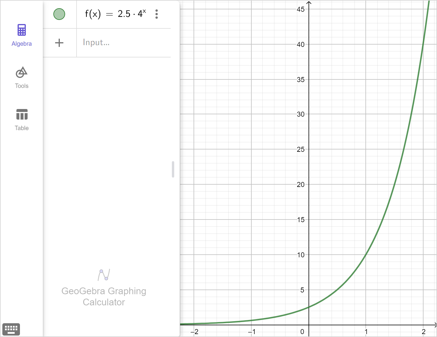
Consider the exponential function y=2.5\left(4\right)^x.

a

Draw the graph of the function.

Worked Solution
Create a strategy

We can identify both the y-intercept and constant factor from the equation since it is of the form y=ab^x. Using these two key features, we can plot other points to the left and right of the y-intercept and connect them with a smooth curve.

Apply the idea

The function has a constant factor of 4 since that is the base of the exponent, and a y-intercept at \left(0,2.5\right) as that is the coefficient.

We can start by plotting the y-intercept and choosing an appropriate scale.

-2
-1
1
2
x
5
10
15
20
25
30
35
40
y

We can see that the function will always be positive, so we don't need any negative y-values.

We know that the constant factor is 4. If we want to go from -2 to 2 on the x-axis, we need to go up to at least 2.5(4)^2=40 on the y-axis.

This would be an appropriate scale as it doesn't have too many labels or tick marks and is easy to read.

-2
-1
1
2
x
5
10
15
20
25
30
35
40
y

Either using a table of values or using the common ratio, we can plot another three points to get a good shape for the graph. Then we can connect the points with a smooth curve.

Reflect and check

When drawing the graphs of exponential functions, we want to be sure the y-intercept is clearly displayed and that the exponential curve is also visible. Be sure to choose a scale for the y-axis that will show all important characteristics. In this case, we chose to scale by 5's, which allows us to read both the y-intercept at 2.5, a second point at \left(1,10\right), the horizontal asymptote at y=0 and the steep slope that all exponential functions have.

b

Check the graph from part (a) using technology.

Worked Solution
Create a strategy

When using a graphing calculator, there will typically be an input bar for functions. We just need to type out the function in the input bar. We need to be careful that we format our input correctly by using the correct buttons.

The GeoGebra calculator has a math input keyboard, but we can also use a computer keyboard.

  • Math input keyboard

    A figure showing how to input y equals 2.5 left parenthesis 4 right parenthesis raised to x. On the left of the figure is the equation y equals 2.5 left parenthesis 4 right parenthesis raised to x. It is followed by a left arrow pointing to a row of 9 keys. Starting from the leftmost key, the labels of the keys are: y, equal sign, 2, decimal point, 5, multiplication sign, 4, a box raised to smaller box, x.
  • Computer keyboard

    Two figures showing 2 ways of how to input y equals 2.5 left parenthesis 4 right parenthesis raised to x. On the left of the first figure is the equation y equals 2.5 left parenthesis 4 right parenthesis raised to x. It is followed by a left arrow pointing to a row of 10 keys. Starting from the leftmost key, the labels of the keys are: y, equal sign, 2, decimal point, 5, left parenthesis, 4, right parenthesis, caret, x. On the left of the second figure is the equation y equals 2.5 left parenthesis 4 right parenthesis raised to x. It is followed by a left arrow pointing to a row of 9 keys. Starting from the leftmost key, the labels of the keys are: y, equal sign, 2, decimal point, 5, asterisk, 4, caret, x.
Apply the idea

The graph should look the same as in part (a). We may need to change the axes or zoom settings to check.

A screenshot of the GeoGebra graphing calculator showing the graph of f of x equals 2.5 times 4 raised to x. Speak to your teacher for more details.

Example 4

Consider the exponential functions f\left(x\right)=2\left(\dfrac{1}{3}\right)^{x} and g\left(x\right)=3\left(\dfrac{1}{2}\right)^{x}.

a

Using a table of values, draw the graph of f\left(x\right) and g\left(x\right) on the same plane.

Worked Solution
Create a strategy

We can identify both the y-intercept and constant factor from each equation since they are of the form y=ab^x. Using these two key features, we can create a table of values of points to the left and right of the y-intercept of each function. We can then plot the points and connect them with a smooth curve.

Apply the idea

First, we can consider the function f\left(x\right). We can see that the function has a constant factor of \dfrac{1}{3} and a y-intercept with coordinates \left(0,2\right).

We can create a table of values with a few points around the y-intercept by substituting in the values x=-3,-2,-1,1,2.

x-3-2-1012
f\left(x\right)541862\dfrac{2}{3}\dfrac{2}{9}

Now, we can consider the function g\left(x\right). We can see that the function has a constant factor of \dfrac{1}{2} and a y-intercept with coordinates \left(0,3\right).

We can create a table of values with a few points around the y-intercept by substituting in the values x=-3,-2,-1,1,2.

x-3-2-1012
g\left(x\right)241263\dfrac{3}{2}\dfrac{3}{4}

Looking at the table of values for f\left(x\right) and g\left(x\right) to determine the scale of the graph, we can see the largest y-value is 54 and we have no negative values of y: the values will continue to decrease, and get closer to the x-axis, but never cross it. So, when plotting the graph, the y-axis has to go up to at least 54 and have an asymptote at y=0.

-3
-2
-1
1
2
x
5
10
15
20
25
30
35
40
45
50
55
y

We can plot the points from our table of values for each function and draw a smooth curve connecting the dots.

Reflect and check

We can see that as x increases, both f\left(x\right) and g\left(x\right) decrease. However, the relative amount of decrease over each interval is different for each function.

b

Determine which function is decreasing at a slower rate.

Worked Solution
Create a strategy

We can compare the constant factors of each function to help determine which function is decreasing slower.

Apply the idea

Considering the functions f\left(x\right)=2\left(\dfrac{1}{3}\right)^{x} and g\left(x\right)=3\left(\dfrac{1}{2}\right)^{x}. We can see that as we approach 0 from the left, for each unit value increase in x, f\left(x\right) is decreasing by a factor of 3, whereas g\left(x\right) is decreasing by a factor of 2.

This means that f\left(x\right) is approaching 0 faster than g\left(x\right). So, we can say that g\left(x\right) is decreasing at a slower rate.

Reflect and check

We can also consider the graph of both functions to confirm that g\left(x\right) is decreasing at a slower rate.

-3
-2
-1
1
2
x
5
10
15
20
25
30
35
40
45
50
55
y

Considering the graph of each function from part (a), we can see that our functions actually intersect at \left(-1,5\right). Before this point, f\left(x\right) is significantly larger than g\left(x\right) at x=-2 and x=-3. But after the point of intersection, g\left(x\right) will always be larger. This confirms that g\left(x\right) is decreasing slower than f\left(x\right).

Example 5

Consider the following exponential functions:

-2
-1
1
2
3
4
x
-9
-8
-7
-6
-5
-4
-3
-2
-1
y
x-2-1012
g(x)-9-3-1-\dfrac{1}{3}-\dfrac{1}{9}
a

Determine which function increases at a slower rate.

Worked Solution
Create a strategy

One way to determine the answer is by comparing the constant factors of the functions. We can find the constant factors by dividing the outputs of two consecutive values of x.

Apply the idea

For f(x), we can use the points (-1, -8) and (0,-2).

b=\dfrac{-2}{-8}=\dfrac{1}{4}

For g(x), we can use the points (-2, -9) and (-1, -3).

b=\dfrac{-3}{-9}=\dfrac{1}{3}

\dfrac{1}{4}<\dfrac{1}{3}, which means f(x) gets multiplied by a smaller factor than g(x). Because of this, f(x) will get closer to 0 faster, so g(x) increases at a slower rate.

Reflect and check

The graphs of f(x) and g(x) are shown below.

-2
-1
1
2
3
x
-9
-8
-7
-6
-5
-4
-3
-2
-1
y

When we look at the graph, we can see g(x) does not seem as steep as f(x) and its curve is more rounded. This is a visual indication that it is increasing at a slower rate.

b

Identify the y-intercept for each function.

Worked Solution
Create a strategy

On the graph, we look for the point where the function intercepts the y-axis. In the table, we look for the point where x=0.

Apply the idea

The y-intercept of f(x) is (0,-2).

The y-intercept of g(x) is (0,-1).

Reflect and check

Now that we know the y-intercept and constant factor for each function, we can build the equations.

f(x)=-2\left(\dfrac{1}{4}\right)^x

g(x)=-1\left(\dfrac{1}{3}\right)^x

Idea summary

We can use the y-intercept and the constant factor to graph an exponential function in the form y=ab^x and identify key features:

  • When a>0 and b>1, the function is increasing at an increasing rate.
  • When a>0 and 0<b<1, the function is decreasing at a decreasing rate.
  • When a<0 and b>1, the function is decreasing at an increasing rate.
  • When a<0 and 0<b<1, the function is increasing at a decreasing rate.
  • When a>0, the range is y>0.
  • When a<0, the range is y<0.

Outcomes

F.IF.B.4

For a function that models a relationship between two quantities, interpret key features of graphs and tables in terms of the quantities, and sketch graphs showing key features given a verbal description of the relationship. Key features include: intercepts; intervals where the function is increasing, decreasing, positive, or negative; relative maximums and minimums; symmetries; end behavior; and periodicity.

F.IF.C.7.E

Graph exponential and logarithmic functions, showing intercepts and end behavior, and trigonometric functions, showing period, midline, and amplitude.

F.IF.C.9

Compare properties of two functions each represented in a different way (algebraically, graphically, numerically in tables, or by verbal descriptions).

F.LE.A.1.B

Recognize situations in which one quantity changes at a constant rate per unit interval relative to another.

F.LE.A.1.C

Recognize situations in which a quantity grows or decays by a constant percent rate per unit interval relative to another.

What is Mathspace

About Mathspace