
7.03 Normal distribution
There are a lot of quantities in real life that exhibit natural variation, for example people's heights, IQ and weights. Even in unnatural processes there can be random errors that result in variation.
For example, consider a manufacturer which produces a chocolate bar with a weight of $50$50 g. It is impossible to make every chocolate bar weigh exactly $50$50 g. But if we weigh $100$100 chocolate bars we would expect the mean value to be very close to $50$50 g. We would also expect most of the measurements to be close to $50$50 g with roughly the same variation above and below $50$50 g, and relatively few measurements that differ significantly from $50$50 g.
If the distribution of chocolate bar weights was displayed in a histogram, the histogram would show a central peak with columns of decreasing height on each side of the mean.

If there could be a vast number of observations put into the histogram with very narrow column widths, the variety of observations would give a bell-shaped histogram that reflects the way in which the frequencies of the observations diminish for values increasingly distant from the mean.
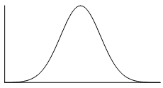
A data set that is symmetrical and bell-shaped about the mean, is said to have a normal distribution.
Two important values are needed to graph or interpret a normal distribution: the mean and the standard deviation.
The mean (represented by the symbol "mu", $\mu$μ) is the location of the maximum density of observations and is where the curve is highest. The curve is symmetrical about the mean. In fact, in a normally distributed data set, the mean, median and mode all take the same value.
The spread of the normal distribution will depend on its variance or the standard deviation (represented by the symbol "sigma", $\sigma$σ) which is the square root of the variance. This will affect how wide and how high the normal distribution is when graphed.
If the standard deviation is low, the proportion of observations near the mean will be high and the curve will be high at the mean value. If the standard deviation is high, the proportion of observations near the mean is reduced and therefore the curve is not so high at the mean.
For example, this distribution curve comes from a data set that has a very small standard deviation, $\sigma=0.2$σ=0.2, and hence is clustered tightly around the mean:

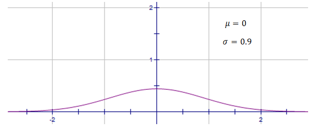
whereas this normal distribution has a larger standard deviation, $\sigma=0.9$σ=0.9, and hence is spread out.
To see how a change in the mean and standard deviation affects the shape of the normal distribution curve, check out the following applet. By moving the sliders around you can vary the mean and standard deviation, and see how the bell curve changes as a result.
Practice questions
QUESTION 1
Which of the following sets of data is approximately normally distributed?
- ABC
QUESTION 2
Which two of the following statements are true for a normal distribution curve?
There are the same number of scores above and below the mean.
AThe curve is symmetrical.
BThe fewest scores lie around the mean.
CThe curve is asymmetrical.
D
QUESTION 3
A sample of professional basketball players is normally distributed and gives the mean height as $199$199 cm with a standard deviation of $10$10 cm.
How tall is a basketball player who is $3$3 standard deviations above the mean?
How tall is a basketball player who is $1.5$1.5 standard deviations below the mean?
Empirical rule
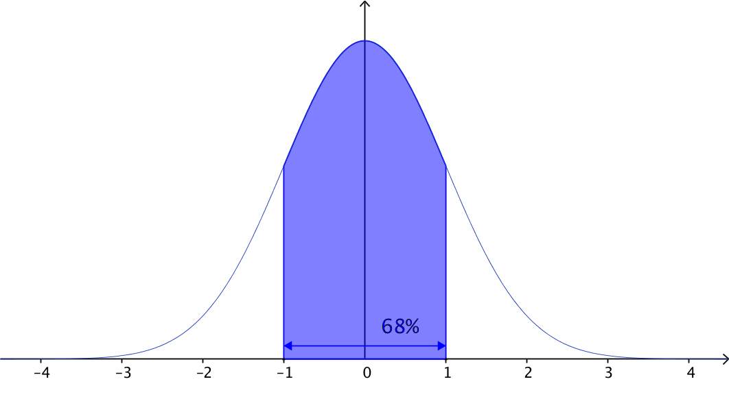
The empirical rule, also known as the $68$68-$95$95-$99.7$99.7$%$% rule, is a way of estimating the way that normally distributed data spreads out. These numbers correspond to the approximate proportion within one, two, and three standard deviations of the mean.
- Approximately $68%$68% of data values lie within $1$1 standard deviation of the mean:
- Approximately $95%$95% of data values lie within $2$2 standard deviations of the mean:

- Approximately $99.7%$99.7% of data values lie within $3$3 standard deviations of the mean:

A normal distribution is symmetrical, so we can use these basic values to find approximations of other regions. For example, as $95%$95% of data values lie within $2$2 standard deviations of the mean, $47.5%$47.5% (half of $95%$95%) will lie between the mean and $2$2 standard deviations above the mean:

We can use a similar trick to conclude that $34%$34% (half of $68%$68%) lies between $1$1 standard deviation below the mean, and the mean itself.
If we add these approximations together, we conclude that $81.5%$81.5% (which is $34%+47.5%$34%+47.5%) of data values lie between $1$1 standard deviation below and $2$2 standard deviations above the mean.
Play around with this applet by moving the endpoints of the shaded region. You will see the percentage of data values lying between the endpoints, and can reveal the percentages of each piece with the toggle:
The estimated proportion tells us the probability that our data will have a value in the given range.
The empirical rule is only an approximation, and we will learn how to use a CAS calculator in the next lesson to more accurately determine probabilities for normally distributed data.
Exploration
Standard deviation is a measure of spread that we can apply to everyday contexts. For example, let's say the mean score in a test was $67$67 and the standard deviation was $7$7 marks. This means that:
- a person with a standard score of $1$1 (that is, $1$1 standard deviation above the mean) would have received a mark of $74$74 (as this is $67+7$67+7).
- a person with a standard score of $-2$−2 (that is, $2$2 standard deviations below the mean) would have received a mark of $53$53 (as this is $67-2\times7$67−2×7).
If we are told that the scores were approximately normally distributed, we could go one step further and determine the percentage of students who scored between $53$53 and $74$74.
The number of students that score between $2$2 standard deviations of the mean would be $95%$95%. The normal distribution is symmetric, so half of $95%$95% of students scored between the mean and two standard deviations below. In other words, $47.5%$47.5% of students scored between $53$53 and $67$67.

Using the same reasoning, we know that half of $68%$68% of students scored between the mean and $1$1 standard deviation above. This means that $34%$34% of students scored between $67$67 and $74$74.

So putting the two percentages together, we can say that $\left(47.5+34\right)%=81.5%$(47.5+34)%=81.5% of students scored between $53$53 and $74$74.
- $68%$68% of data values lie within $1$1 standard deviation of the mean.
- $95%$95% of data values lie within $2$2 standard deviations of the mean.
- $99.7%$99.7% of data values lie within $3$3 standard deviations of the mean.
Since the normal distribution is symmetric, we can halve the interval at the mean to halve the percentage of data values.
Practice questions
QUESTION 4
The grades in a test are approximately normally distributed. The mean mark is $60$60 with a standard deviation of $2$2.
Between which two scores does approximately $68%$68% of the results lie symmetrically about the mean? Write both scores on the same line, separated by a comma.
Between which two scores does approximately $95%$95% of the results lie symmetrically about the mean? Write both scores on the same line, separated by a comma.
Between which two scores does approximately $99.7%$99.7% of the results lie symmetrically about the mean? Write both scores on the same line, separated by a comma.
QUESTION 5
The following figure shows the approximate percentage of scores lying within various standard deviations from the mean of a normal distribution. The heights of $600$600 boys are found to approximately follow such a distribution, with a mean height of $145$145 cm and a standard deviation of $20$20 cm. Find the number of boys with heights between:

$125$125 cm and $165$165 cm
$105$105 cm and $185$185 cm
$85$85 cm and $205$205 cm (to the nearest whole number)
$145$145 cm and $165$165 cm
$165$165 cm and $185$185 cm (to the nearest whole number)
QUESTION 6
In a normal distribution, what percentage of scores lie between $2$2 standard deviations below and $3$3 standard deviations above the mean? Use the empirical rule to find your answer.