INVESTIGATION: Time series data

The skills and tools required to analyse time series data can be combined with the statistical investigation process to analyse real-world data.

A step-by-step example of an investigation into Perth petrol prices in 2016 is provided. While the data used is from 2016, the analytical process remains relevant and applicable to current problems.

Read through the example to understand the process. This knowledge can then be applied to investigate a problem using more recent data, such as predicting the price of petrol at a local station in 2030.

The statistical investigation process

Reminder - these steps form a rigorous and complete statistical investigation process:

1. Identify a problem
2. Collect or obtain data
3. Analyse data
4. Interpret and communicate results

The problem

The objective is to understand the fuel price cycle for Perth.

The statistical question

When is the cheapest time to buy petrol in Perth and what is the expected price for unleaded petrol on the cheapest day next week?

For the context of this investigation, the analysis is set in late February or early March 2016. Therefore, "next week" refers to the period from Monday, 29th February to Sunday, 6th March 2016.

Collecting the data

Data for time series analysis can be obtained from online government resources that track average price movements. The ACCC website is a useful source for prices in all major Australian cities.

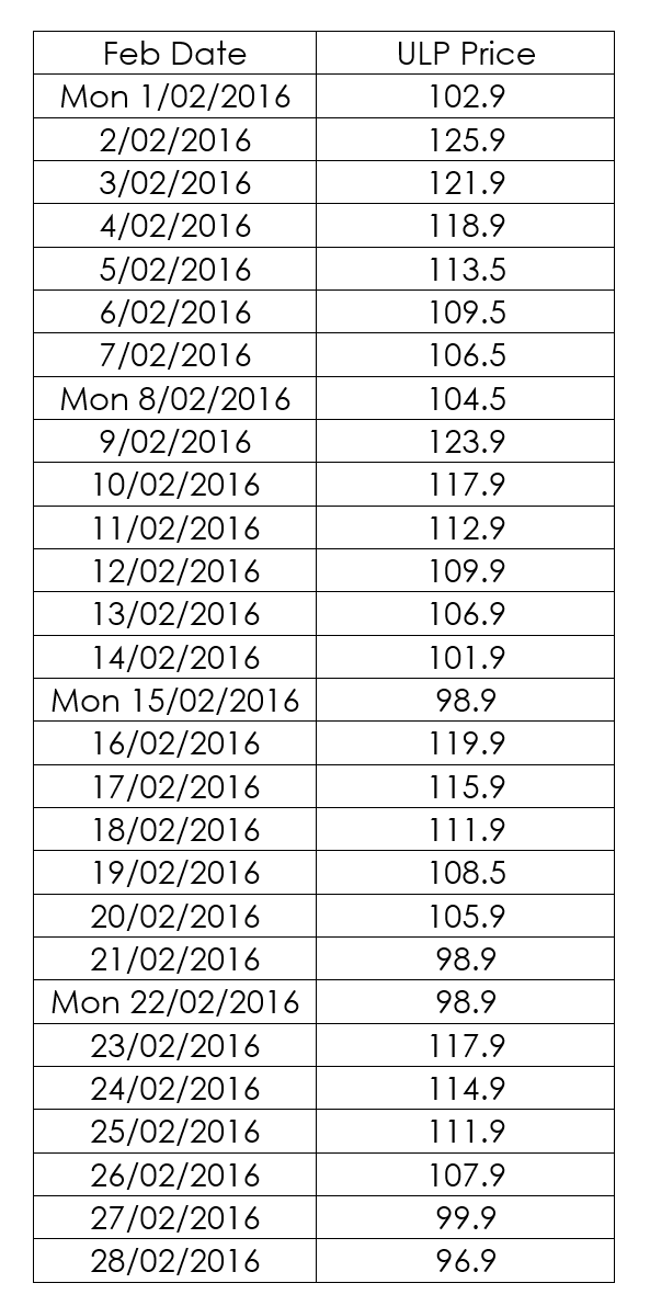
For this investigation, historical data were sourced from Perth's 'FuelWatch' website. After downloading the February 2016 data file, filters were applied to isolate the price cycle at a single location: the Caltex petrol station in Balcatta.

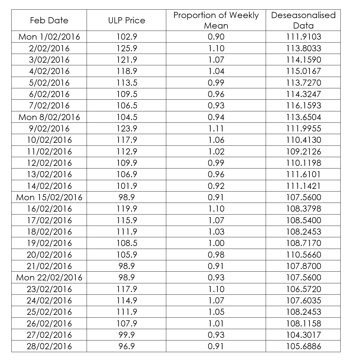
The resulting unleaded petrol prices for each day in February 2016 at this station are shown:

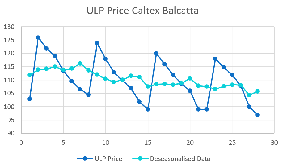
Use a spreadsheet to create a line graph of this data.

Analysing the data

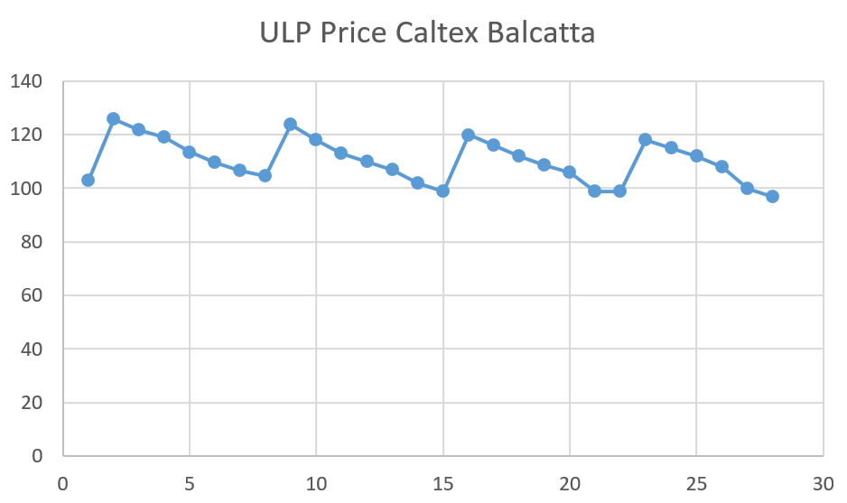
The time series plot reveals two key features: a distinct 7 -day cycle and a slight declining trend, as the price decreases slightly each week.

This visual analysis indicates that fuel is cheapest on a Monday. Therefore, the optimal day to purchase unleaded petrol is Monday, 29th February. To forecast the price for that specific day, the data requires further analysis.

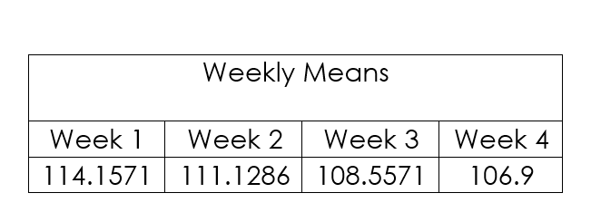
The first step is to calculate the mean for each of the four weeks:

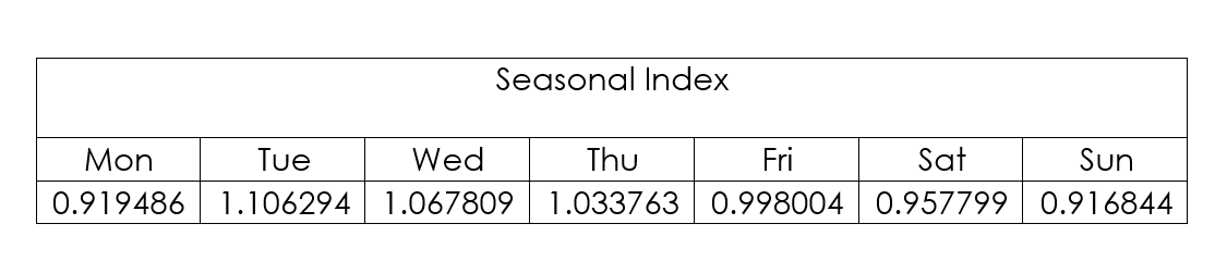
Then, calculate each proportion of the weekly means and the seasonal indices.

Then, deseasonalise the data.

Graph the raw data along with the deseasonalised data on the same axes to observe the smoothing effect.

The next step is to determine the equation of the least-squares regression line for the deseasonalised data, where t = 1 is Monday, 1st February.

The resulting least-squares regression line is:

y=-0.3278t+114.9397

The regression equation can now be used to predict the price for Monday, 29th February 2016.

Note that t = 29 in this case.

y=105.4324

Re-seasonalise the prediction by multiplying the forecast value by the seasonal index for Monday.

105.4324\times0.9195=96.95 cents/litre

Interpreting and communicating the result

Based on the model, the predicted price for ULP at Caltex in Balcatta on Monday, 29th February 2016, 96.95 cents/litre. This forecast's reliability is considered high because it involves interpolation, falling within one cycle of the original data. For context, the actual price on that day was 93.9 cents/litre.

 

Questions 

1. If a prediction was made for the Balcatta Caltex for Wednesday 9th March, 2016, what comment should be made on the reliability of the prediction?
2. What underlying assumptions are made when using this model to predict future values?
3. What could be the reason(s) for the spike in petrol prices on Tuesdays?
4. Suggest some real-life events that could make predictions from historical records, such as these, unreliable.