When we have a set of univariate data, it often happens that most of the measurements will be clustered close to the mean value with the density of the observations falling off as distance away from the mean increases. Results of this kind displayed in a histogram show a central peak with columns of decreasing height on each side of the mean.
The normal distribution is a special type of continuous probability distribution. It is often called the "bell curve" because of the shape of the graph. The normal distribution is important in statistics because it can be used to describe many natural variables. For example, for a large population a person's height, arm span, and IQ are each variables which demonstrate an approximate normal distribution.
The bell curve is symmetrical about the mean (which is where the peak of the bell occurs) and it has the property that the mean, mode and median are all equal.
Probability distributions that display the distinctive bell curve together with its properties are described as being "normally distributed".

The shape of the normal distribution will depend on its mean ($\mu$μ) and standard deviation $(\sigma)$(σ). The mean is where the graph peaks. To draw a normal distribution graph we only need the mean and standard deviation values.
For the normal distribution, the mean is exactly in the middle, so $50%$50% of the values are above the mean and $50%$50% of the values are below the mean.
The width of the bell curve is approximately $3$3 standard deviations left and right of the mean as most scores lie within that range.
The normal distribution formula
The probability density function describing the normal distribution function is written in terms of the mean $(\mu)$(μ) and standard deviation $(\sigma)$(σ):
$\phi\left(x\right)=\frac{1}{\sigma\sqrt{2\pi}}e^{-\frac{\left(x-\mu\right)^2}{2\sigma^2}}$ϕ(x)=1σ√2πe−(x−μ)22σ2
We won't be using this formula to find the probabilities. Instead, we will primarily be using our available technology on our calculators which we will demonstrate in our next lesson.
Exploration
Assume that a population is normally distributed with mean $\mu$μ and standard deviation $\sigma$σ. Use the following applet to discover what happens to the graph as we change the mean and standard deviation.
- What do you notice about the shape of the graph when we change the mean?
- What happens to the shape of the graph as $\sigma$σ gets closer to $0$0?
For example, this distribution curve comes from a data set that has a very small standard deviation, $\sigma=0.2$σ=0.2, and hence is clustered tightly around the mean:

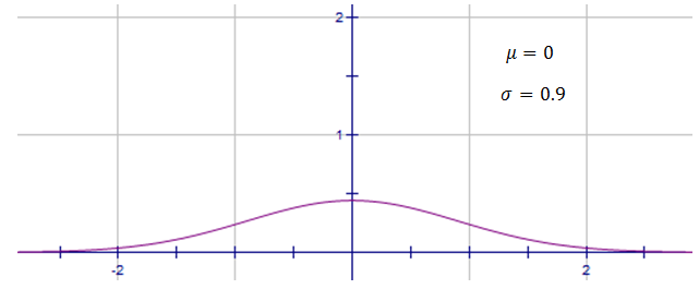
This normal distribution has a larger standard deviation, $\sigma=0.9$σ=0.9, and hence is quite spread.
Practice questions
Question 1
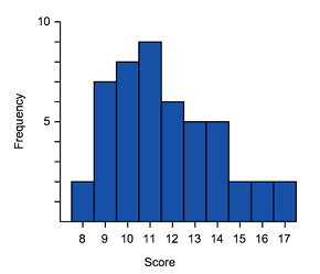
Which of these histograms is approximately normally distributed?
 A
A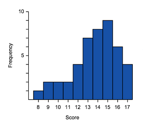 B
B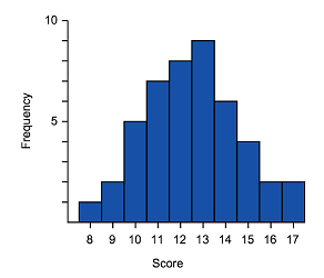 C
C
Question 2
Which two of the following statements are true for a normal distribution?
The spread of the normal distribution changes depending on the mean.
AA higher mean will result in a skewed curve.
BThe mean, median and mode all have the same value.
CThe spread of the normal distribution changes depending on the standard deviation.
D
The empirical rule
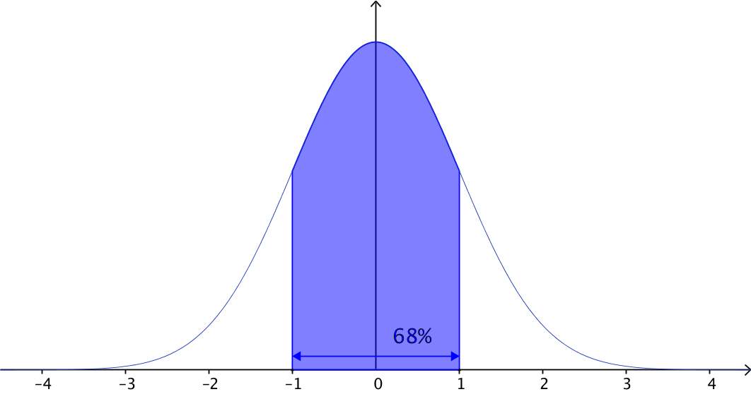
The empirical rule, also known as the $68-95-99.7%$68−95−99.7% rule, is a way of estimating the way that normally distributed data spreads out. These numbers correspond to the approximate proportion within one, two, and three standard deviations of the mean.
- Approximately $68%$68% of scores lie within $1$1 standard deviation of the mean:
- Approximately $95%$95% of scores lie within $2$2 standard deviations of the mean:

- Approximately $99.7%$99.7% of scores lie within $3$3 standard deviations of the mean:

A normal distribution is symmetrical, so we can use these basic values to find approximations of other regions. For example, as $95%$95% of scores lie within $2$2 standard deviations of the mean, so $47.5%$47.5% (half of $95%$95%) will lie between the mean and $2$2 standard deviations above the mean:

We can use a similar trick to conclude that $34%$34% (half of $68%$68%) lies between $1$1 standard deviation below the mean, and the mean itself.
If we add these approximations together, we conclude that $81.5%$81.5% (which is $34%+47.5%$34%+47.5%) of scores lie between $1$1 standard deviation below and $2$2 standard deviations above the mean.
Play around with this applet by moving the endpoints of the shaded region. You will see the percentage of scores lying between the endpoints, and can reveal the percentages of each piece with the toggle:
The empirical rule is only an approximation, and better approximations exist. For example, a better approximation for the area between $1$1 standard deviation below and above the mean is
$68.268949213...%$68.268949213...%
An exact value is impossible to write down, like many other important numbers in mathematics, so we need to approximate somewhere. For now, this is just a good place to start thinking about the distribution.
Exploration
Standard deviation is a measure of spread that we can apply to everyday contexts. For example, let's say the mean score in a test was $67$67 and the standard deviation was $7$7 marks. This means that:
- a person who was $1$1 standard deviation above the mean would have received a mark of $74$74 (as this is $67+7$67+7).
- a person who was $2$2 standard deviations below the mean would have received a mark of $53$53 (as this is $67-2\times7$67−2×7).
If we're told that the scores were approximately normally distributed, we could go one step further and determine the percentage of students who scored between $53$53 and $74$74.
The number of students that score between $2$2 standard deviations of the mean would be $95%$95%. The normal distribution is symmetrical, so half of $95%$95% of students scored between the mean and two standard deviations below. In other words, $47.5%$47.5% of students scored between $53$53 and $67$67.
Using the same reasoning, we know that half of $68%$68% of students scored between the mean and $1$1 standard deviation above. This means that $34%$34% of students scored between $67$67 and $74$74.
So putting the two percentages together, we can say that $\left(47.5+34\right)%=81.5%$(47.5+34)%=81.5% of students scored between $53$53 and $74$74.
- $68%$68% of scores lie within $1$1 standard deviation of the mean.
- $95%$95% of scores lie within $2$2 standard deviations of the mean.
- $99.7%$99.7% of scores lie within $3$3 standard deviations of the mean.
Remember, since the normal distribution is symmetrical, we can halve the interval at the mean to halve the percentage of scores.
Practice questions
Question 3
The image shows the distribution of females’ heights in a population. Use the image to help you complete the following statements.

$34%$34% of females lie between $157$157 cm and $163$163 cm and $\editable{}$% of females lie between $163$163cm and $169$169cm.
$1$1 standard deviation = $\editable{}$ cm.
question 4
The following figure shows the approximate percentage of scores lying within various standard deviations from the mean of a normal distribution. The heights of $600$600 boys are found to approximately follow such a distribution, with a mean height of $145$145 cm and a standard deviation of $20$20 cm. Find the number of boys with heights between:

$125$125 cm and $165$165 cm
$105$105 cm and $185$185 cm
$85$85 cm and $205$205 cm (to the nearest whole number)
$145$145 cm and $165$165 cm
$165$165 cm and $185$185 cm (to the nearest whole number)
question 5
The operating times of phone batteries are approximately normally distributed with mean $34$34 hours and a standard deviation of $4$4 hours. Answer the following questions using the empirical rule:
Approximately what percentage of batteries last between $22$22 and $42$42 hours?
Approximately what percentage of batteries last between $30$30 hours and $42$42 hours?
Any battery that lasts less than $22$22 hours is deemed faulty. If a company manufactured $51000$51000 batteries, approximately how many batteries would they be able to sell? Round your answer to the nearest integer.

