As we have seen, a Discrete Random Variable, or DRV for short, is when each outcome in a random experiment is assigned a number.
A Continuous Random Variable, or CRV for short, is when we examine the outcomes over an interval for a random experiment.
An easy way to think about it is this: we count the outcomes for a DRV and we measure the outcomes for a CRV.
Now that we know the difference between a DRV and CRV, we want to take a closer look at DRVs, and in particular, we want to look at the distribution of the probabilities.
The Probability Distribution of a Discrete Random Variable
For a DRV, each outcome is assigned a probability.
For example, let's say we toss a coin twice and we're interested in how many tails we see.
Firstly we can define our DRV. Let $X$X be the number of tails in a two coin toss.
We then know that $X$X can take on the values of $0$0, $1$1 or$2$2.
The probability distribution for X will show us the probabilities for each of these outcomes. An easy way to do that for this example is to look at a tree diagram.

We'll now examine our tree diagram and tabulate the probabilities.
| $x$x | 0 | 1 | 2 |
|---|---|---|---|
| $P(X=x)$P(X=x) | $\frac{1}{4}$14 | $\frac{2}{4}$24 | $\frac{1}{4}$14 |
What we've just created is the probability distribution for the random variable $X$X.
How can we represent a probability distribution for a DRV?
There are a few ways we represent a probability distribution for a DRV.
- We can create a table of values. This is the most common method.
- We can create a function. You will see this very soon.
- We can draw a graph.
The graph of a probability distribution for a DRV.
The graph of a probability distribution of a DRV is a probability histogram.
Either of these two graphs can be used to represent the DRV X that we were discussing earlier.

Uniform vs Non-Uniform DRVs
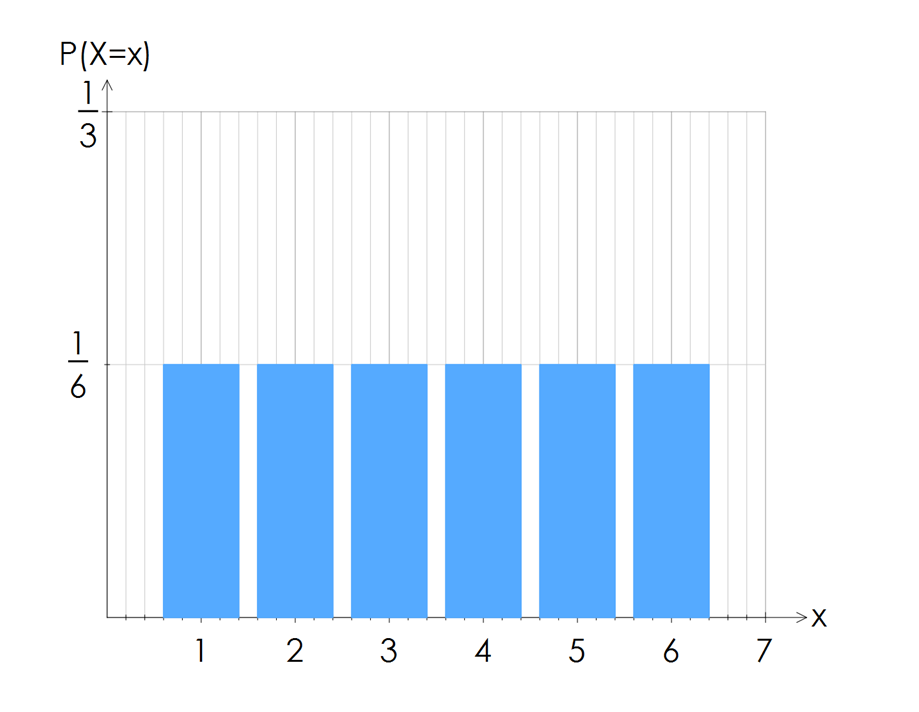
A uniform DRV is when all outcomes of the experiment are equally likely.
For example, when you roll a dice once, the probability of rolling a $1$1,$2$2, $3$3, $4$4,$5$5 or $6$6 are all equally likely, or uniform.
The probability histogram below of one roll of the dice shows this uniform shape nicely.

A non-uniform DRV is when not all outcomes are equally likely. This is the vast majority of DRVs that we'll see.
The Properties of a Probability Distribution of a DRV
If we examine what appears to be a probability distribution, either in a table, a graph or a function, we need to make sure each of the following three properties apply:
- All outcomes are numerical and discrete - this means we can't have categorical or continuous numerical data.
- The probabilities of all possible outcomes add to $1$1 - this makes sense when you think about it, if they didn't all add up to $1$1 then we must be missing one of the outcomes or have one of the probabilities wrong.
- The probability $p$p of all outcomes is greater than or equal to $0$0 and less than or equal to $1$1, that is $0\le p\le1$0≤p≤1.
Worked Examples
Question 1
Is the following a probability distribution?
| $x$x | $2$2 | $4$4 | $6$6 | $8$8 |
|---|---|---|---|---|
| $p\left(x\right)$p(x) | $0.2$0.2 | $0.4$0.4 | $0.6$0.6 | $0.8$0.8 |
No
AYes
B
Question 2
Consider the following table.
| $x$x | $2$2 | $4$4 | $5$5 | $6$6 | $7$7 |
|---|---|---|---|---|---|
| $P$P$($($X=x$X=x$)$) | $0.1$0.1 | $0.25$0.25 | $0.3$0.3 | $0.15$0.15 | $0.2$0.2 |
Identify which conditions for a discrete probability distribution are evident in the table.
Select all that apply.
$X$X is discrete numerical
A$\Sigma P\left(x\right)=1$ΣP(x)=1
B$0\le P$0≤P$\left(x\right)\le1$(x)≤1
CNone of the conditions
DTherefore, does this table represent a discrete probability distribution?
No
AYes
B
Question 3
Consider the following graph.
Identify which conditions for a discrete probability distribution are evident in the graph.
Select all that apply.
$X$X is discrete numerical
A$\Sigma P\left(x\right)=1$ΣP(x)=1
B$0\le P$0≤P$\left(x\right)\le1$(x)≤1
CNone of the conditions
DTherefore, does this graph represent a discrete probability distribution?
Yes
ANo
B